GEOD
log
Drawing a stratigraphic log with the log command
The log command is used to draw a stratigraphic log.
Summary
- Basic syntax
- Patterns
- Indentations
- Bed boundaries
- linecolor
- linewidth
- linehidden
- teeth
- wave
- zigzag
- karst
Basic syntax
The log command is used to draw stratigraphic logs. For lithological patterns, it fully reuses the capabilities of the pattern command.
To insert a log and define its different lithological units, the following syntax is used:
  log
      unit e1 "label1"
          --> pattern definition instructions
      unit e2 "label2"
          --> pattern definition instructions
      ...
      unit en "labeln"
          --> pattern definition instructions
Each lithological unit is declared with the keyword unit. The parameters e1, e2, ..., en are the respective thicknesses of the units, expressed in metres, and label1, label2, ... labeln are the labels displayed on the right. These labels must be enclosed in double quotation marks and may contain any kind of character, including spaces and tabs. Text-formatting instructions such as bold, italic, superscript, or subscript may also be inserted, as presented in this section.
Figure 1 gives a first example of a log built with the log command. The following instructions were inserted into the script:
  log
      unit 30 "a"
      unit 60 "b"
      unit 35 "c"
      unit 15 "d"
      unit 15 "e"
      unit 15 "f"
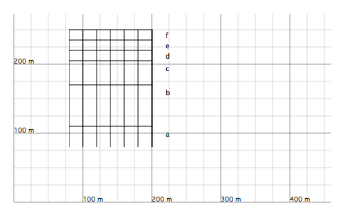
Figure 1. Elementary stratigraphic log composed of 6 units.
By default, the stratigraphic column is 120 metres wide. The text on the right is separated from the column by a distance of 20 metres.
Patterns
By default, each unit is displayed with a lithological pattern made of vertical bars spaced every 20 metres. This pattern can of course be customized. To do so, all the instructions of the pattern command may be used. These instructions must follow the unit instruction, as indicated above.
For example, for the unit labelled "a", one may write:
  unit 30 "a"
      circle
      size 6
      levels 2
      alternate
      novertical
      nohorizontal
      spacing 15
      markerscale 1.3 1
      fillcolor yellow
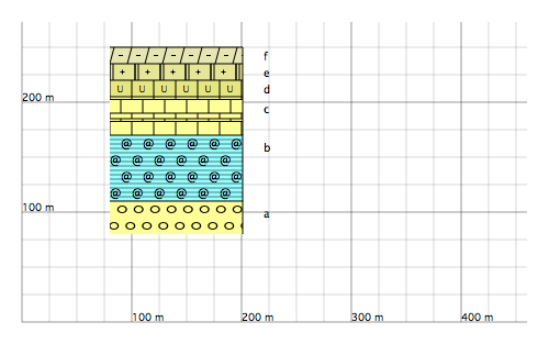
Figure 2. Same stratigraphic column as in figure 1, but with lithological patterns applied.
A predefined pattern may also be specified by using the keyword with followed by the name of the predefined pattern.
  unit 30 "a"
      with pa
where pa is the name of a predefined pattern, defined for example by:
  set p1 to pattern
      circle
      ...        --> continuation of the pattern definition instructions
Indentations
In logs, it is common to display information about rock hardness and resistance to erosion. Softer beds are drawn recessed, whereas harder beds are shown in relief. The log command makes it possible to create such indentations by means of the hard instruction. This subcommand may be used in three different syntactic forms, with one, two, or three arguments.
The first form creates logs with rectangular indentations:
hard d
where d is a parameter measuring rock hardness. It also corresponds to the indentation value.
- if d > 0, the bed is drawn in relief, and its outcropping side is shifted d metres to the right.
- if d < 0, the bed is recessed, and its outcropping side is shifted d metres to the left.
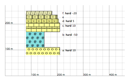
Figure 3. Same log as in figure 2, but with indentations produced by the simple form of the hard instruction. The corresponding hard instructions are shown next to it.
Another form of hard uses two arguments:
hard d c
In this form, hard creates curved indentations.
The second parameter, c, controls the curvature of the bed. The top and base are symmetrical.
- if c > 0, the bed is convex to the right, and the top and base are more eroded than the middle part.
- if c < 0, the bed is concave to the right, and the middle part is more eroded than the top and base.
The erosion difference between the central part and the top and base is roughly equal to half of c.
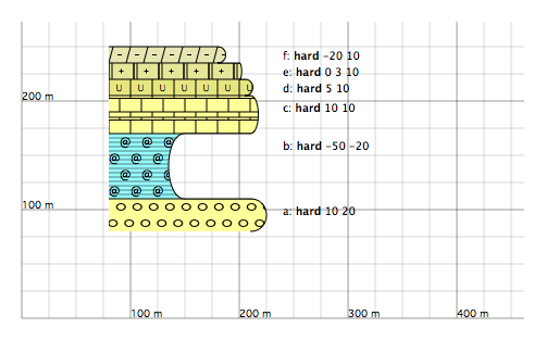
Figure 4. Same log as in figure 3, but with curved bed margins. The corresponding hard instructions are shown next to it.
Finally, when followed by three arguments, the hard subcommand makes it possible to produce more realistic logs: the bed margins remain curved, but the base and top are no longer symmetrical.
hard d m t
where m and t are the curvature parameters at the base and at the top, respectively. When one of these parameters is positive, the curve is convex to the right; when it is negative, the curve is convex to the left.
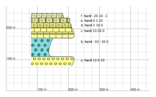
Figure 5. Same log as in figure 4, but with different curvature at the top and at the base. The corresponding hard instructions are shown next to it.
Bed boundaries
The log command also makes it possible to control the appearance of bed boundaries, especially their thickness and colour. More complex boundary morphologies may also be drawn.
linecolor
The linecolor subcommand draws the bed boundary located at the top of the unit in a colour other than black. Its syntax is the same as that of the other colour-modification subcommands. See this section for more details.
For example, to draw bed boundaries in red, as in figure 5, one inserts:
linecolor red
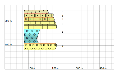
Figure 6. Same log as in figure 5, except that the bed boundaries are drawn in red with a linecolor red instruction.
linewidth
The linewidth instruction sets the thickness of the line used to draw the bed boundary located at the top of the unit:
linewidth e
where e is the thickness, expressed in metres.
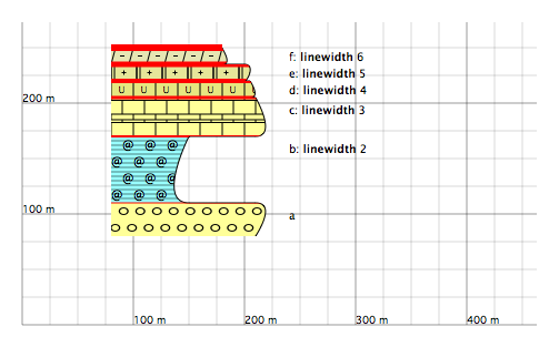
Figure 7. Same log as in figure 6, but with bed boundaries of different thickness. The corresponding linewidth instructions are shown next to it.
linehidden
In some cases, it is useful to hide bed boundaries, especially when the transition from one bed to the next is gradual. This is possible with the linehidden instruction:
linehidden
linehidden hides the bed boundary located at the top.
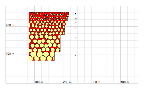
Figure 8. Stratigraphic log with 6 beds and progressive decrease of marker size upward. Bed boundaries are hidden with the linehidden instruction.
teeth
The teeth instruction replaces unit boundaries with angular, saw-tooth lines.
In its simplest form, this subcommand is used without argument:
teeth
In this case, it draws a crested line with an amplitude of 8 metres and a period of 40 metres.
In some cases, teeth may be followed by a single argument:
teeth h
where h is the half-amplitude of the line.
In its most complete form, with two arguments, one writes:
teeth h p
where the additional parameter p is the half-period of the line.
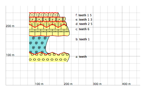
Figure 9. Examples of unit boundaries drawn with teeth. The corresponding instructions are shown next to them.
wave
The wave subcommand is the sinuous equivalent of teeth. It draws unit boundaries as waves or undulations. Its syntax therefore works in the same way. See the paragraph above, replacing teeth by wave.
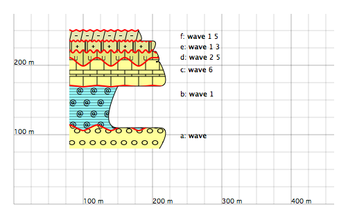
Figure 10. Examples of unit boundaries drawn as waves with wave. The corresponding instructions are shown next to them.
zigzag
The zigzag subcommand generates oblique unit boundaries, with or without zigzag-shaped indentations. Such figures are used when the transition from one unit to another does not occur at the same time everywhere. They may therefore represent lateral facies variations.
As usual, this instruction applies to the boundary located at the top of the unit. It may take 0, 1, or 2 arguments.
In its simplest form, this subcommand draws a toothed line with two teeth, inclined to the left. The line has two steps, a lower one on the left and a higher one on the right. These two steps are offset by 10 metres relative to one another and are centred on the top of the unit. In practice, this subcommand also affects the position of the top of the unit: it is raised by 5 metres on the right and lowered by 5 metres on the left.
zigzag
zigzag may also be followed by one argument:
zigzag d
where d is the offset value between the lower and upper steps, expressed in metres.
When d > 0, the oblique line rises to the right. When d < 0, the oblique line rises to the left.
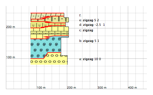
Figure 11. Examples of oblique toothed unit boundaries produced by zigzag instructions. The corresponding instructions are shown next to them.
Finally, this instruction may take two parameters:
zigzag d n
where n is the number of teeth.
When n = 0, the zigzag subcommand draws a simple oblique line.
karst
The karst subcommand draws an irregular line that may be used to represent eroded contacts, such as those found on former karstified surfaces.
The syntax of this instruction is similar to that of teeth and wave. The subcommand may be used with 0, 1, or 2 arguments. In its complete form:
karst h p
h denotes the half-amplitude of the line, whereas p is the half-period.
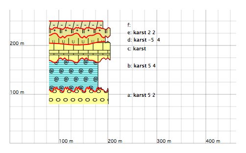
Figure 12. Examples of unit boundaries drawn as irregular lines with karst. The corresponding instructions are shown next to them.
Labels
Labels are the pieces of text displayed next to the units. Each unit has its own label. These labels share some features with the text command. In particular:
- to insert a line break into a label, use the character |. See this section.
- to write some words in bold or italics, or as subscript or superscript, use the backslash character. See this section.
fontsize
The fontsize instruction sets the size of the font used for the text.
fontsize s
where s is expressed in metres.
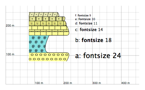
Figure 13. Illustration of the fontsize instruction.
Layout
x and y
A log may be moved on the drawing figure. To do this, use the instructions:
  x ...
  y ...
where the ... must be replaced by the coordinates of the lower-left corner of the log.
This instruction may be placed anywhere in the definition of the log. The quickest way to use it is to click on the figure while pressing the command key.
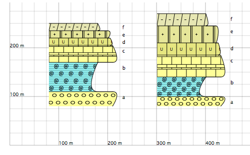
Figure 14. Example of compared logs with two stratigraphic columns side by side. The second one is shifted relative to the first by an instruction such as x 300 y 80.
logwidth
The logwidth instruction sets the width of the stratigraphic column, which is 120 metres by default:
logwidth w
where w is expressed in metres.
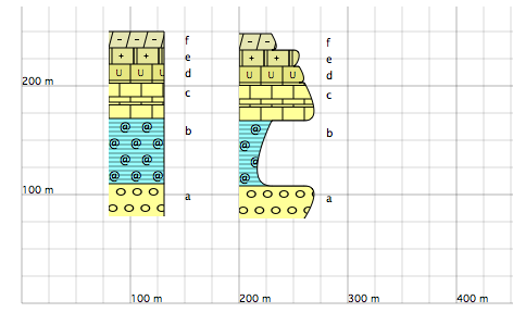
Figure 15. Same stratigraphic logs as in figure 2 for the left log and as in figure 5 for the right log, but with a narrower column produced by logwidth 50.
margin
The margin subcommand specifies the width of the space between the stratigraphic column and the label area:
margin s
where s is expressed in metres.
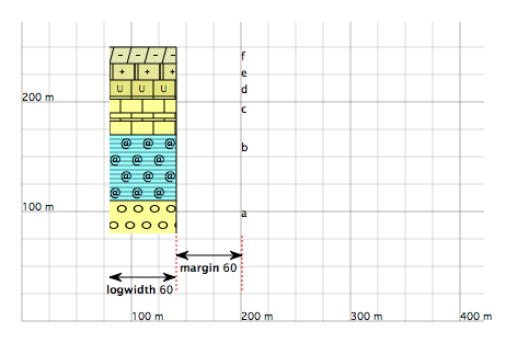
Figure 16. Adjusting the space between the column and the text area with margin 60.
textwidth
The textwidth instruction modifies the width of the text area:
textwidth s
where s is expressed in metres. By default, the text area is 200 metres wide.
This command is sometimes necessary when labels contain very long lines that may otherwise be truncated.
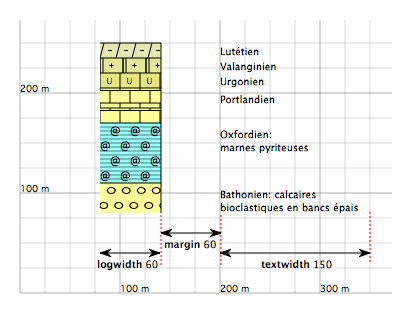
Figure 17. The textwidth instruction used to adjust the size of the text area.
Other options
Drawing interbed lines
The current version of GEOD does not provide a specific command to draw interbed lines. Moreover, for compared logs, it is often easier to draw them manually with the mouse.
For example, in figure 17, instructions of the following type were used:
  line
      x ... y ...
      ...
      dotted color black width 2
to draw these interbed lines.
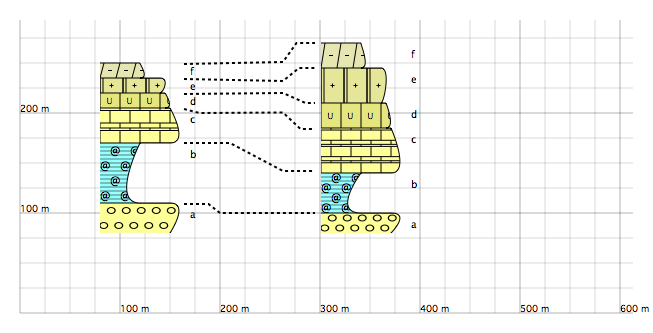
Figure 18. Compared logs with interbed lines.
Drawing a graduated scale
A log is often accompanied by a vertical graduated scale. To display such a scale, one uses a line command together with a graduate instruction. For example, for the graduated line to the left of the log in figure 18, the following instructions are used:
  line
      65 80
      dir 90 199
      graduate left 50
      arrow last gypsum filled length 5
      color black
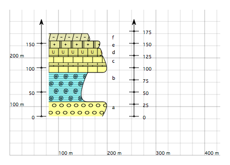
Figure 19. Stratigraphic log accompanied by a graduated scale, on the left and on the right.
Drawing a pluton
In some cases, one may need to draw an intrusive body, such as a granitic pluton, cutting across the stratigraphic column. To do so, one uses a fill command enclosed within a clip ... unclip command. In addition, the fill motif must be accompanied by a fore instruction.
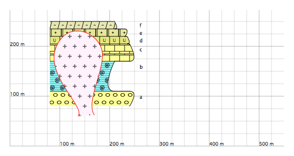
Figure 20. Stratigraphic column cut by a granitic pluton.
Drawing a dyke or sill
Other intrusive bodies, such as dykes and sills, may also be represented on the stratigraphic column.
For these objects, it is sufficient to use a line command offset with an offset command, with a lithological pattern applied by a pattern command. Here again, a fore instruction must be used with the pattern command.
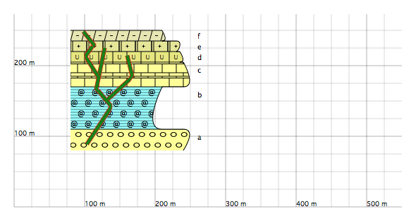
Figure 21. Stratigraphic column cut by a dyke network.