GEOD

pattern (3)

Lithological patterns: the pattern command (3)

This section deals with multi-layer patterns, the definition and use of a pattern library, and several additional options related to the pattern command.

Summary

• Multi-layer patterns
• Building and using a pattern library
• Variable-thickness layers
• Other options
• fore
• debug

Multi-layer patterns

Up to this point, only single-layer patterns have been described. To summarize, such patterns are made of transverse and intermediate bars that divide the space between two layer boundaries into a number of cells. These cells may be alternating or not, and each cell may contain at most one marker. Many instructions are available and allow a wide variety of motifs to be generated. However, certain things cannot be achieved with single-layer patterns:

• several different marker types cannot be used together,
• markers cannot be superimposed on the bars,
• and gradients cannot be drawn between two colours other than white, for example from red to yellow.

All these limitations are removed by multi-layer patterns. A multi-layer pattern may be described as the superposition of several patterns, each one having its own settings.

A multi-layer pattern is defined with the keyword over, each over instruction introducing a new layer:

  pattern
      ...      -- instructions for the base layer
      over     -- declare a new layer
      ...      -- instructions for this layer
      over     -- another layer

The instructions defining each new layer must be placed after the keyword over. Any number of layers may be used, and they are drawn in the order in which they are introduced: the first layer forms the base, and the last one is the topmost layer.

As an illustration, the full set of instructions used to produce the motif in Figure 1 is given below:

  pattern
      circle
      filled
      markercolor red
      color red
      spacing 40
      size 8

Note the use of the patternoffset subcommand in the second layer. This instruction is what allows the triangles of the second layer to be drawn directly above the transverse bars of the first layer. Without it, the blue triangles would sit directly above the red dots.

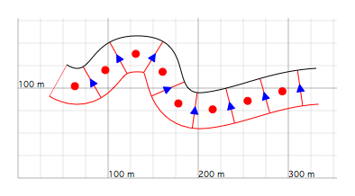
Figure 1: Two-layer motif produced by the instructions above. The first layer, made of small red dots and red bars, is covered by a second layer made of small blue triangles.

×

To create a background gradient between two colours other than white, two additional layers may be used. For example, to draw the gradient shown in Figure 2, one may write:

  pattern
      fillcolor yellow
      novertical

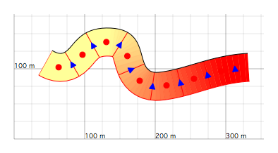
Figure 2: The same motif as in Figure 1, but with a background gradient from yellow to red. The motif now consists of four layers.

Building and using a pattern library

The same motif will often be used several times in a geological cross-section, especially when a given formation appears in several compartments. Rather than repeating the full definition of a motif each time, it is more efficient to use a predefined style.

To define a lithological pattern in advance, one uses the set command with the following syntax:

  set patternName to pattern
      ...

The dots must be replaced by the usual definition instructions of the pattern command. All the subcommands introduced for pattern, including multi-layer definitions with over, may be used here.

The parameter patternName is chosen by the user and gives a name to the predefined motif.

To use a predefined motif, one simply writes with followed by its name:

  pattern
      with patternName

For example, the motif shown in Figure 3 is drawn with a predefined pattern as follows:

  set j3 to pattern
      fillcolor yellow
      levels 10
      width 0.4
      alternate
      sequence ( 1 1 1 4 2 3 )
  over
      alternate
      levels 2
      char @
      size 13
      spacing 30
      novertical
      nohorizontal

This predefined motif, named j3, can then be used by any pattern command simply by writing:

  pattern with j3

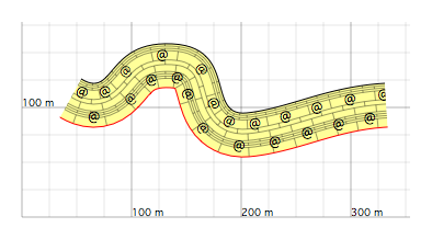
Figure 3: Two-layer motif drawn from a predefined pattern.

Predefined motifs may also be stored in files other than the script currently being edited. To use such external pattern files, the include command can be used in the main script.

Variable-thickness layers

In many situations, layers do not have a constant thickness. This may happen for three different reasons:

1. the layer has variable thickness because sedimentation took place over a restricted depositional area, such as a pond, lake, arm of the sea, or lagoon. In that case, the layer has a lens-shaped geometry, with beds resembling stacked shallow dishes and gradually thinning toward the margins.
2. the layer has variable thickness because sedimentation occurred in a basin with irregular topography. Beds are thicker where the depth, that is, the available accommodation space, was greatest. The oldest deposits must also occur in these deeper areas. The layer is then angularly unconformable on its substratum.
3. the layer has variable thickness because its beds have been partly removed by erosion.

In a geological cross-section, an experienced observer should be able to recognize from the pattern why a given layer has variable thickness.

By default, when a layer does not have constant thickness, the pattern command draws a motif made of lens-shaped levels or beds. Implicitly, GEOD assumes the first case, that of lenticular deposits.

The pattern command can automatically draw motifs corresponding to the two other cases as well.

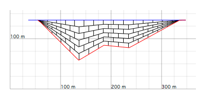
Figure 4: Variable-thickness layer with a lenticular shape. The mother curve is shown in blue, and the daughter curve was obtained by a variable offset using the offset command.

For a layer in angular unconformity on its substratum, use the instruction:

  discordant

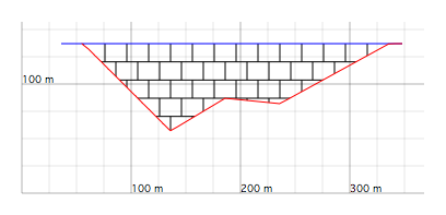
Figure 5: Variable-thickness layer in angular unconformity on its substratum. The motif was drawn with the instruction discordant.

For a layer that has been partly truncated by erosion, use the instruction:

  eroded e

where e is the initial thickness of the layer. This parameter is optional and may be omitted. By default, GEOD assumes an initial thickness of 100 metres.

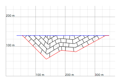
Figure 6: Variable-thickness layer partly truncated along its margins by erosion. The motif was drawn with the instruction eroded 80.

Other options

fore

Figure 7 shows a layer cut by a dyke. The dyke was drawn using a line command and an offset command. Its interior was coloured using a pattern command with the instruction fillcolor blue.

A close look at the figure reveals a problem in the rendering of the dyke: the boundaries of the yellow layer, the mother curve and the daughter curve, are not covered by the dyke.

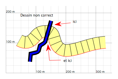
Figure 7: Dyke intrusion through a folded layer. The drawing is not correct because the layer boundaries are not covered by the dyke.

This is not a bug in GEOD, but rather a consequence of the way the program draws a cross-section:

• GEOD first draws all the motifs, whether lithological motifs produced by pattern or more general fill motifs produced by fill,
• then, in a second step, GEOD draws all the other graphical objects, such as lines, curves, and text, in the order in which they appear in the script.

This procedure ensures a good rendering of lines and curves. Without it, the mother and daughter curves of a layer would be partly eaten away by their associated motif.

Nevertheless, exceptions can be made with the instruction:

  fore

This subcommand tells GEOD to treat the motif like any other graphical object of the line or curve type. This corrects the drawing problem. On the other hand, the boundaries bordering the motif may then become partly masked by it.

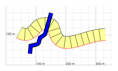
Figure 8: The drawing is now correct thanks to the use of the fore instruction. In return, part of the borders, although drawn with 4-pixel-thick lines, has been lost.

debug

The debug subcommand is useful while developing a cross-section. It cancels all the other instructions defined for the pattern command and reveals the skeletal framework of the motif. The motif is then represented by a set of small red segments connecting corresponding points of the mother curve and the daughter curve.

These are the points calculated by the offset algorithm, used by the offset command, or by the shift algorithm, used by shift. These are also the very points that the pattern command uses to compute the motif. The debug instruction can therefore help diagnose problems related to slow rendering or incorrectly computed layers.

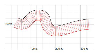
Figure 9: Motif drawn with the debug instruction.