GEOD
line
Lines
Lines are built as a sequence of connected segments. They are especially useful for drawing topographic profiles, faults, dykes, and layer boundaries when the available data are numerous and precise.
Summary
- Construction
- Basic syntax: x and y
- The dir subcommand
- The fix subcommand
- The rel subcommand
- Graphic attributes
- Dotted and dashed lines
- The dashed subcommand
- The color subcommand
- The width subcommand
- The backcolor subcommand
- Orientation and curvilinear coordinates
- The extendfirst and extendlast subcommands
- The hextendfirst and hextendlast subcommands
- The u0 subcommand
- The graduate subcommand
- Advanced graphic attributes
- Line patterns
- Customizing line patterns
- Arrows
- Predefined line styles
- Variable styles with style
- Discontinuous lines with gap
- Attaching points and lines
- The name subcommand
- The tie subcommand
- Topographic profile
- Example: constructing fault blocks
- Advanced options
- The nocrossing subcommand
- The segnb and seglen subcommands
- The control subcommand
- The hidden subcommand
Construction
Basic syntax
To define a line, simply enter the coordinates of its successive points.
  line
      x 65.0 y 70.0
      x 109.0 y 82.0
      x 136.0 y 99.0
      x 164.0 y 95.0
      x 204.0 y 89.0
      x 221.0 y 99.0
      x 256.0 y 81.0
      x 283.0 y 82.0
      x 298.0 y 76.0
      width 2
      color blue
This produces the following line:
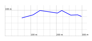
Figure 1: Drawing a polyline with the line command.
The syntax can be simplified by omitting x and y.
  line
      65.0 70.0
      109.0 82.0
      ...
A line can also be constructed quickly with the mouse. Hold down the Command key and click on the desired location. GEOD then inserts the coordinates automatically into the script editor.
The dir subcommand
It is sometimes useful to construct a line step by step, starting from a point and using distance and angle data.
This can be done with the dir subcommand:
dir angle distance
This subcommand takes two arguments:
- a direction, expressed as an angle in degrees. Angles are measured counterclockwise. A direction of 0 corresponds to a horizontal movement from left to right.
- a distance.
  line x 100 100
      dir 45 100
      dir -45 100
      dir 45 100
      dir -45 100

Figure 2: Drawing a polyline with a sequence of dir instructions.
In other words, this method is equivalent to using polar coordinates.
The fix subcommand
Another way to define a line is with the fix subcommand. It works in the same way as dir:
fix angle distance
but here the angle is given as a deviation measured relative to the direction of the preceding segment. A value of 0 extends the line in the same direction, a value of 90 turns the line at right angles to the right, and a value of -90 turns it at right angles to the left.
The angular deviation is always measured while moving along the segment from left to right.
This subcommand is particularly efficient for constructing geometric figures.
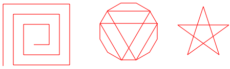
Figure 3: Drawing geometric figures with fix.
The rel subcommand
A line can also be constructed from relative displacement data with the rel subcommand, whose syntax is:
rel deltax deltay
where deltax and deltay indicate the horizontal and vertical distances to be travelled from the previous point in order to position the new point.
Thus,
rel 160 -60
tells GEOD to insert a new point located 160 metres to the right and 60 metres below the previous point.
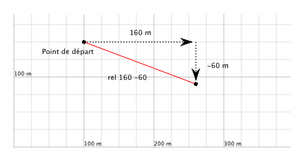
Figure 4: Drawing a line with rel.
Graphic attributes
Dotted and dashed lines
GEOD provides many options to control the appearance of a line.
- dotted draws a dotted line.
- dashed draws a dashed line.
- dot and square are also available. They are mainly useful for debugging, because they display the points actually stored in the memory of GEOD.
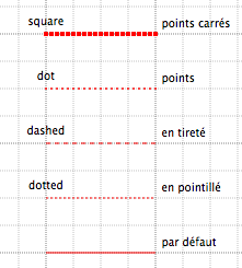
Figure 5: Display options for a polyline.
Customizing dashes with dashed
With the dashed subcommand, the dash length can be adjusted precisely. dashed can be used in three different ways:
1. Default dashed line:
dashed
draws dashes made of solid segments 4 pixels long separated by 3-pixel gaps.
2. Custom solid segment length:
dashed len1
draws dashes with solid segments of length len1 pixels, separated by 3-pixel gaps.
3. Custom solid and gap lengths:
dashed len1 len2
draws dashes with solid segments of length len1 pixels followed by gaps of length len2 pixels.
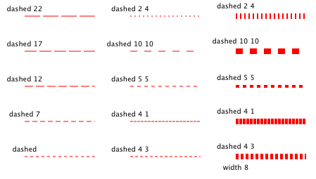
Figure 6: Adjusting dash length with dashed.
The color subcommand
The line color can be modified with the color subcommand.
This subcommand can be used either:
- with a color name such as black, gray, or yellow. See the color list here.
- or with three numbers between 0 and 1 specifying the red, green, and blue components.
color blue
color 0.5 0.5 1.0
The width subcommand
The width subcommand specifies the line thickness in pixels.
width 0.1
This draws a very fine line with a thickness of 0.1 pixel.
The backcolor subcommand
backcolor specifies a background color for the line drawing. It is generally used together with dashed, dotted, or dot.
  backcolor yellow
      color red
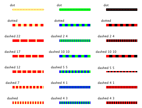
Figure 7: Dashed lines with backcolor.
Orientation and curvilinear coordinates
In GEOD, every line has a default orientation:
- from the first point defined in the script, which is the starting end,
- to the last point, which is the terminal end.
This orientation defines the curvilinear coordinate system. Its values therefore range from zero at the starting end to the total line length at the terminal end.
The figure below illustrates two lines drawn with GEOD. One is defined from left to right, the other from right to left. Circles mark the starting ends, while crosses indicate the points of curvilinear coordinate 300. Thick marks show the points calculated by GEOD at curvilinear coordinates 100 and 200.
In GEOD, the curvilinear coordinate of a point is denoted by the letter u.
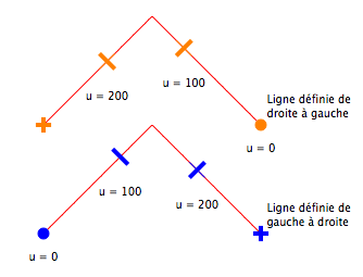
Figure 8: Orientation and curvilinear coordinates.
The extendfirst and extendlast subcommands
It is sometimes useful to extrapolate a line beyond its starting or ending point. This can be done with the extendfirst and extendlast subcommands. The extrapolation direction follows the direction of the end segments.
  line ...
      extendfirst 50
extends the line by 50 metres before the first point.
Using extendfirst and extendlast has no effect on the scale of the curvilinear coordinates, as shown in the figure below. The lines are extended at both ends without changing the position of points at curvilinear coordinates 100 and 200.
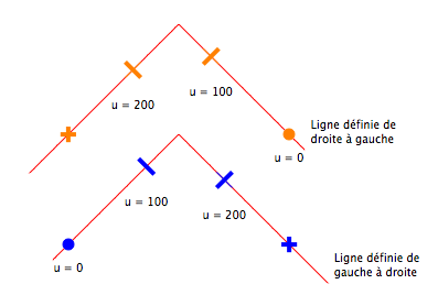
Figure 9: The extendfirst and extendlast subcommands.
The hextendfirst and hextendlast subcommands
These two commands, like extendfirst and extendlast, extend the curve beyond its ends, but only in a horizontal direction.
In practice, these instructions are mainly useful for animations. hextendfirst and hextendlast are then needed to impose boundary conditions during terrain compression.
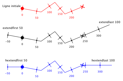
Figure 10: The extendfirst, extendlast, hextendfirst, and hextendlast subcommands used to extend a line at its ends.
The u0 subcommand
The u0 subcommand changes the origin of the curvilinear coordinate scale of a line.
u0 100
moves the origin of the curvilinear coordinate scale 100 metres beyond the initial end of the curve.
A negative value may also be given to u0.
  extendfirst 100
  u0 -50
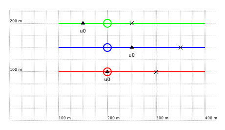
Figure 11: Illustration of the u0 command. On the three lines shown, the origin of the curvilinear scale has been changed. Circles mark the original starting points, and crosses indicate the terminal ends. The three lines have been extended with extendfirst and extendlast. Black triangles show the new origins of the curvilinear scales (u0 0 for the red line, u0 50 for the blue line, and u0 -50 for the green line). Each small square corresponds to 25 metres in the figure.
As will be seen later, this command is particularly useful for sliding blocks against one another and modelling thrusts and nappes.
The graduate subcommand
The graduate subcommand displays tick marks along the entire line, making its curvilinear coordinates visible. It is useful during the construction of a cross-section when assembling lines associated by curvilinear coordinates, for example with an instruction of the form tie lineName at u ....
This command can be used in two forms, a short form and a long form.
In the short form, simply write:
graduate
GEOD then marks the line every 50 metres.
In the long form, write:
graduate value
where value specifies the spacing of the graduations.
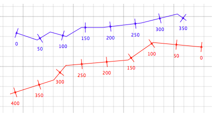
Figure 12: The graduate command used to display the curvilinear coordinates of a line.
By default, GEOD displays the graduations below the line. To display them above the line, write:
graduate above
or, to change the spacing to 100 metres for example,
graduate above 100
The graduations can also be displayed on the left:
graduate left
or on the right:
graduate right
Advanced graphic attributes
Line patterns
GEOD can also be used to draw geological maps and structural diagrams. For this purpose, it provides a set of conventional line patterns to represent different categories of structural elements such as normal faults, reverse faults, thrusts, nappes, and fold axes.
The available line patterns are illustrated in the figure below.
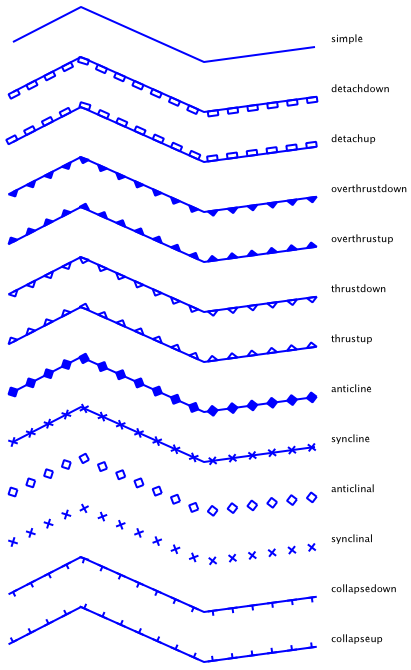
Figure 13: Line patterns and their corresponding subcommands. The lines are defined from left to right.
To use a particular line pattern, simply call the corresponding subcommand. For example, to draw a line bordered by small barbs on its right side, or downward in the drawing when the line is oriented from left to right, use the collapsedown instruction.
  line ...
      collapsedown
Main predefined line styles:
- simple — draws a simple line
- anticlinal — draws an anticline axis in a keystone style
- anticline — same, but with a connecting line between the diamonds
- synclinal — draws a syncline axis in a stitching style
- syncline — same, but with a line connecting the cross symbols
- thrustup — draws a thrust fault, with the left side overriding the right side
- thrustdown — draws a thrust fault, with the left side underthrust by the right side
- collapseup — draws a normal fault, with the downthrown block on the right
- collapsedown — same, with the downthrown block on the left
- overthrustup — draws the front of a thrust sheet, with the nappe on the right
- overthrustdown — same, but with the nappe on the left of the line
- detachup — draws a detachment fault, with the displaced block on the left of the line
- detachdown — same, with the displaced block on the right of the line
Customizing line patterns
Line patterns can be customized with two subcommands: patternspace and patternsize.
patternspace controls the spacing between the symbols along the line. It is followed by a value specifying the spacing, in metres, between the markers that make up the pattern.
patternsize controls the size of the pattern symbols. It can be used in two ways:
1. With a single argument indicating the size of the symbols in metres.
patternsize 10
2. With two arguments giving the symbol size, in metres, on the left and right sides of the line respectively. This form is useful for constructing asymmetric line patterns.
patternsize 3 12
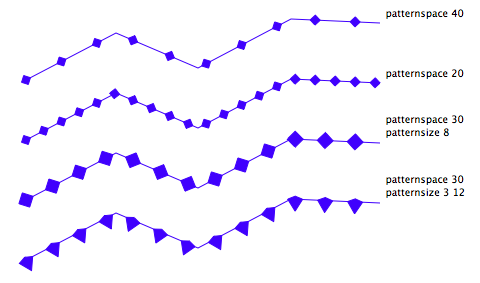
Figure 14: The patternspace and patternsize subcommands used to customize line patterns. Here, line patterns suitable for representing anticline axes on a structural sketch are shown. The asymmetric pattern defined with patternsize can be used to indicate an overturned fold.
Arrows
GEOD can draw arrows at the ends of lines using the arrow instruction. This instruction can be used on its own or followed by additional arguments.
1. Arrow at both ends:
  line ...
      arrow both
draws a line with an arrow at each end.
2. Arrow at the starting end:
arrow first
3. Arrow at the terminal end:
arrow last
or simply:
arrow
draws an arrow at the final end.
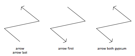
Figure 15: The arrow subcommand.
By default, GEOD draws a standard arrow as illustrated above. Other arrow styles are also available.
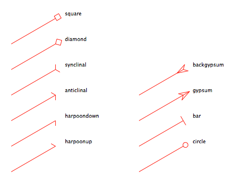
Figure 16: The different arrow styles available in GEOD.
For example, to draw an arrow shaped like a spearhead, write:
  line ...
      arrow last gypsum
A shorter, though less readable, syntax can also be used:
  line ...
      arrow last 9
where 9 is the code for the spearhead arrow style.
Available arrow styles include:
- arrow ... square — square arrowhead — code 6
- arrow ... diamond — diamond arrowhead — code 5
- arrow ... synclinal — snake-tongue arrow — code 4
- arrow ... anticlinal — standard arrow — code 3
- arrow ... harpoondown — harpoon with the head pointing downward — code 2
- arrow ... harpoonup — harpoon with the head pointing upward — code 1
- arrow ... gypsum — spearhead arrow — code 9
- arrow ... backgypsum — same, but reversed — code 10
- arrow ... bar — bar marker — code 8
- arrow ... circle — circular marker — code 7
GEOD also provides additional subcommands to customize arrows:
- length, which sets the arrow size.
length 30
This specifies an arrow 30 pixels long.
- angle, which modifies the angle between the arrow branch and the line on which it is attached.
angle 20
This increases the angle by 20 degrees.
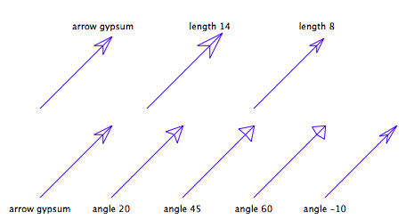
Figure 17: The angle and length instructions used to customize arrow appearance.
- filled, which fills the inside of the arrow. This subcommand takes no argument.
filled
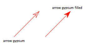
Figure 18: The filled instruction used to fill the inside of an arrow.
Finally, the instructions width, dotted, dashed, and color also affect the drawing of arrows. In contrast, backcolor has no effect on arrows.
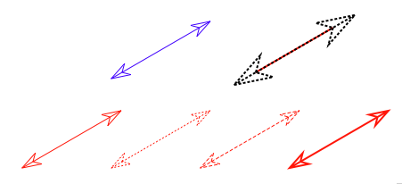
Figure 19: Effect of width, dotted, dashed, color, and backcolor on arrows and lines.
Predefined line styles
Several lines in the same figure may share the same attributes. Rather than redefining the same parameters for each curve, it is often more convenient to use a predefined style. A style is defined with the instruction set ... to style and is applied to a line with the keyword with.
For example, to define a style:
  set monStyle to style
      color blue dashed 5 3
      width 3 backcolor cyan
To apply this style to a line, simply write:
  line ...
      with monStyle
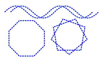
Figure 20: Applying a predefined line style to four lines.
Variable styles: the style subcommand
GEOD can vary the appearance of a line as a function of its curvilinear coordinate. For example, it is possible to draw lines with variable thickness or color. This is done with the style subcommand.
The style subcommand is followed by a list of attribute specifications, such as width, color, and others, enclosed in parentheses. Each specification is followed by the keyword upto and a curvilinear coordinate value, defining the interval over which that specification remains valid.
Each upto ... instruction must be followed by a comma or semicolon, except for the last one before the closing parenthesis.
Example:
  line ...
      style
      (
      width 3 upto 100,
      width 1 upto 150,
      hidden upto 200,
      width 3 color blue upto 300,
      width 1 dashed
      )
The figure below illustrates the result of such a style definition.
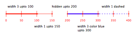
Figure 21: Drawing a line with a style varying according to curvilinear coordinates.
Note that the style subcommand can also create discontinuous lines with the keyword hidden, which masks a portion of the line. Another way to achieve this is described below.
Discontinuous lines: the gap subcommand
Discontinuous lines can also be constructed with the gap instruction. This keyword separates the different parts of the line.
Example:
  line
      100 100 dir 0 100
      gap
      300 150 dir 45 100
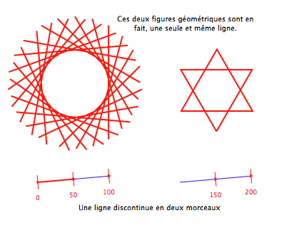
Figure 22: Example of discontinuous lines constructed with the gap instruction.
Attaching points and lines
GEOD allows points and lines to be attached to one another. Thus, it is possible to:
- define a new point with the point command on a given line,
- or, conversely, construct a new line with the line or bezier command from a set of points defined by the point command.
The tie subcommand is what makes it possible to associate lines and points with one another. This is an essential way to constrain the construction of a cross-section. It can be used, for example, to place markers on a topographic profile.
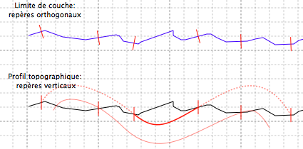
Figure 23: The tie subcommand used to place markers on a line.
There is an important subtlety in the way GEOD draws points attached to a line. If the supporting line is a topographic profile and has been declared as such by naming it topo, then the markers are drawn vertically. If the supporting line is a layer boundary, the markers are drawn perpendicular to the line.
The name subcommand
In order to attach an object to a given line, the line must first be named. This is done with the name subcommand.
For example:
  line ...
      name ordo1
assigns the name ordo1 to the line currently being defined.
The tie subcommand
To place a point on a line, use the tie subcommand:
  line
      ...
      name maLimiteDeCouche
In the example above, a marker point is defined on the curve named maLimiteDeCouche, at curvilinear coordinate u = 60.
A point can be attached to a line from several kinds of specifications.
1. From a curvilinear coordinate:
tie lineName at u curvilinear_coordinate
To place a point at the beginning of a line:
tie lineName at u 0
To place it at the terminal end, it would normally be necessary to know the total line length. Instead, the symbol \* or the keyword last can be used:
tie lineName at u *
tie lineName at u last
2. From a horizontal coordinate x:
tie lineName at x horizontal_coordinate
3. From a vertical coordinate y (altitude):
tie lineName at y vertical_coordinate
4. From a depth value:
Depth is a distance measured downward from a topographic profile.
tie lineName at depth vertical_coordinate
See the section below on the topographic profile for how this works.
Topographic profile
In a cross-section, the topographic profile plays a special role. It is the reference line used for depth measurements. In GEOD, lines and points can be constructed from depth data.
To do so, it is necessary to indicate which line is used as the topographic profile. This is done by giving it the name topo:
  line ...
      name topo
To indicate that a point lies at a depth of 100 metres, one may write:
  point
      x 200
      tie topo at depth 100
To construct a line from depth data, the same principle applies:
  line
      x 200 tie topo at depth 50
      x 300 tie topo at depth 30
      x 400 tie topo at depth 70
If the topographic profile is later modified, GEOD automatically updates all points and lines constructed from depth data.
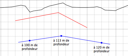
Figure 24: The black line is a topographic profile, defined as such in GEOD with the instruction name topo. The other objects, blue points and red and blue lines, are constructed from depth data.
Example: constructing fault blocks
The combination of the tie, dir, and fix instructions makes it possible to construct rigid volumes that can then be moved and made to slide on certain surfaces.
An example is given below with the sliding of blocks above a listric fault. The reconstruction with GEOD clearly shows that the sliding of these blocks necessarily creates voids at their base, which are then filled by drag and flow of ductile evaporitic deposits shown in pink.
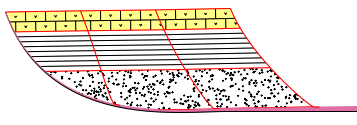
Figure 25: The listric fault and the fault blocks in the initial stage.
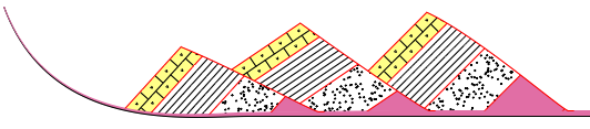
Figure 26: The listric fault and the fault blocks in the final stage.
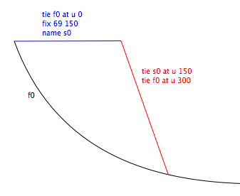
Figure 27: Construction of a block using the tie and fix subcommands.
Advanced options
The nocrossing subcommand
nocrossing removes all portions of a line that form a loop. This subcommand exists, but it is only rarely needed in practice.
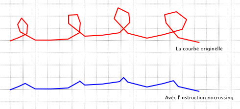
Figure 28: The nocrossing subcommand.
The segnb and seglen subcommands
GEOD inserts intermediate points between the points explicitly defined by the user. These intermediate points may be called nodes. For the display of a line itself, they are not especially useful, but they become important when computing an offset curve with the offset command or when drawing lithological patterns.
In principle, the more intermediate points there are, the more accurate the drawing becomes, though at the cost of longer computation time.
The number of inserted points depends on the internodal distance. The larger this distance, the more intermediate points are inserted. In all cases, GEOD inserts at least one intermediate node.
By default, GEOD inserts one intermediate point every 5 metres. However, if the internodal distance is too large, GEOD limits the number of inserted points, with a default maximum of 50.
In most cases, there is no need to change the default settings. However, this is possible with segnb and seglen.
seglen sets the spacing, 5 metres by default, between two intermediate points. Thus,
  line ...
      seglen 100
constructs a line made of points spaced 100 metres apart. This may be sufficient when working at the scale of 1:1,000,000.
segnb sets the maximum number of segments formed by the intermediate points between two nodes. Since the default value is 50, it can be modified as follows:
  line ...
      segnb 100
In all cases, it is not possible to specify a value greater than 1000.
A schematic view of the algorithm is given below, followed by examples of its application.
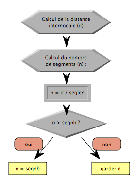
Figure 29: The algorithm used to calculate the number of intermediate points inserted between two curve nodes.
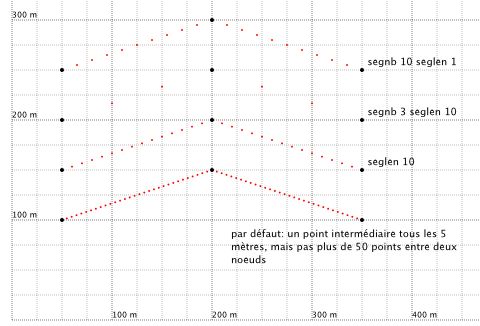
Figure 30: The segnb and seglen subcommands.
It is also possible to modify the default seglen and segnb parameters for all lines in GEOD through the Preferences. This is generally not recommended, since it changes the rendering of all cross-sections.
The control subcommand
It is sometimes useful to display the control points, or nodes, used to build a line.
This can be done via the menu Cross Sections -> Show Control Points or with the Control icon. However, this displays the nodes of all lines defined in the cross-section, which may make the figure difficult to read.
GEOD offers another subcommand, control, which displays only the nodes belonging to a specific line.
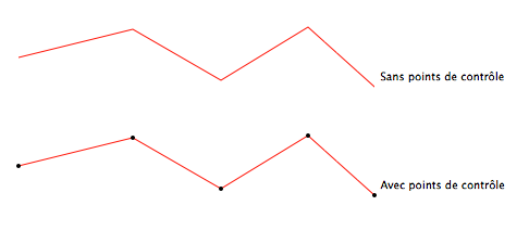
Figure 31: The control subcommand used to display the nodes of a specific line.
The hidden subcommand
The hidden subcommand hides the line. It takes no argument.
hidden