GEOD

pattern (1)

Lithological patterns: the pattern command (1)

GEOD includes a very complete and efficient command, called pattern, for drawing the lithological patterns of geological layers. In accordance with standard geological practice, these patterns are drawn so that they follow the layer boundaries. Many options make it possible to customize their appearance and to create a wide variety of patterns.

Summary

• The pattern command
• Presentation
• Syntax
• Bars
• levels
• vspacing
• graded
• sequence
• novertical
• nohorizontal
• spacing
• alternate
• oblique
• double
• period
• spacing2
• patternoffset
• width
• dashed
• dotted
• base

The pattern command

Presentation

The pattern command is used to decorate geological layers with repetitive motifs that follow their contours. To use this command, two conditions must be satisfied.

• first, two layer boundaries are required, commonly called the roof and the base of the layer in geology. These boundaries are curves that may be produced by the commands line, bezier, offset, shift, or bezoff.
• second, one of these curves, called the daughter, must be derived from the other, called the mother, by a geometric operation, either an offset with offset or a translation with shift.

In principle, it is therefore not possible to place a pattern directly between two independent Bézier curves or between two independent polylines. The reason is that the pattern command needs to establish a point-by-point correspondence between the two curves in order to calculate the motif. This can be done easily only when one curve is geometrically derived from the other.

Later on, the bezoff command will provide a useful workaround. It is in fact an offset curve disguised as a Bézier curve, and it therefore makes it possible to place a pattern between two curves as if they were genuine Bézier curves.

Syntax

In its full form, the pattern command requires at least one argument: the name of the daughter curve.

  pattern daughter

where daughter must be replaced by the name of the daughter curve, previously defined with a name instruction.

The result is shown below.

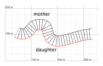
Figure 1: Default lithological pattern drawn between the daughter curve and its mother curve. Here, the daughter curve was produced by a downward offset of 40 metres using the offset command.

×

By default, GEOD draws a simple pattern made of vertical bars spaced 10 metres apart. Because of the curvature of the boundaries, this spacing is measured along the median line, which is invisible on screen, between the mother and daughter curves.

The command pattern daughter may be inserted anywhere in the script. It may appear either before or after the definitions of the mother and daughter curves.

If the last curve defined before the pattern command is the daughter curve, then the syntax can be simplified further. There is no need to specify the daughter by name, and it may even remain unnamed. In that case, simply write:

  bezier
      x ... y ...

Between the definition of the daughter curve and the pattern command, other objects may be defined, such as text in the example above. The only restriction is that they must not be new curve definitions made with line, bezier, offset, shift, or bezoff.

So far, only a very simple pattern has been considered. In practice, the pattern command is followed by a series of subcommands that control its appearance.

Bars

Bars are one of the main elements used to recognize lithological patterns. They may be horizontal, vertical, or oblique, regularly or irregularly spaced, periodic, or arranged in alternating layouts. GEOD provides a wide range of subcommands to control their appearance.

levels

The levels instruction draws internal stratification lines. Its syntax is:

  levels n

where n is the number of stratified levels between the roof and the base of the layer.

For example, the instruction levels 4 produces a pattern composed of four internal stratification levels.

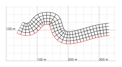
Figure 2: Drawing a pattern with four stratified levels using levels 4.

With levels, the thickness of the internal strata is proportional to the thickness of the layer itself, as shown below.

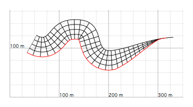
Figure 3: In a variable-thickness layer, here tapering into a wedge, the strata created with levels are themselves of variable thickness.

vspacing

Like levels, the vspacing instruction introduces internal stratification lines. Its syntax is:

  vspacing e

where e sets the thickness of an elementary stratum in the pattern.

For example,

  vspacing 16

tells GEOD to draw strata 16 metres thick. But if the layer itself is 40 metres thick, GEOD will in practice draw three strata: the first two will each be 16 metres thick, while the last one, adjacent to the daughter curve, will be only 8 metres thick.

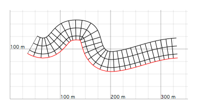
Figure 4: Effect of vspacing 16 on a layer 40 metres thick. Since 40 is not a multiple of 16, GEOD truncates the last stratum, the one adjacent to the daughter curve.

Just like levels, vspacing adapts the thickness of the strata to the total thickness of the layer.

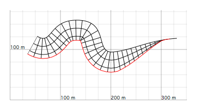
Figure 5: Effect of the same instruction, vspacing 16, on a variable-thickness layer.

If a pattern command is followed by both a levels instruction and a vspacing instruction, even if they contradict each other, then vspacing takes precedence.

graded

In sedimentary series, it is common to observe an upward evolution in bed thickness, either positive, with beds becoming thicker upward, or more commonly negative, with beds becoming thinner upward.

Such arrangements can be mimicked with the graded instruction:

  graded f

where f is a strictly positive parameter controlling the relative evolution of stratum thickness from the mother curve to the daughter curve.

• if f > 1, the beds become progressively thicker,
• if f < 1, the beds become progressively thinner,
• if f = 1, the graded instruction has no effect.

The farther f is from 1, the more pronounced the increase or decrease in stratum thickness.

For example,

  graded 0.5
  levels 15

creates a pattern made of 15 strata whose thickness decreases from the mother curve to the daughter curve.

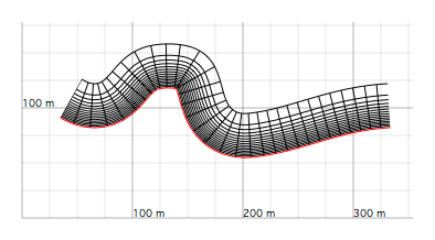
Figure 6: Pattern with strata thinning from the mother curve to the daughter curve, produced by graded 0.5.

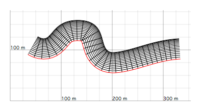
Figure 7: Same idea, but with graded 1.5. The strata become thicker near the daughter curve.

sequence

In sedimentary successions, strata are often organized into groups called sequences, which form motifs that repeat, more or less regularly, along the vertical direction.

For example, a layer may consist of a recurring sequence composed of a thick bed overlain by a thinner bed.

The sequence instruction creates patterns that simulate the repetition of such sequences.

For a sequence with n terms, the syntax is:

  sequence ( e1 e2 ... en )

where e1, e2, ..., en are positive numbers measuring the relative importance of each term in the sequence. What matters here is not their absolute value, but their relative proportions. In its current version, GEOD cannot accept sequences containing more than 24 terms.

For example, to create the motif shown below, composed of a two-term sequence, one thick bed followed by one thin bed, one may write:

  sequence ( 5 1 )

The first number, 5, means that the first term of the sequence is five times more important than the second. The same motif could equally well be produced by sequence (25 5) or sequence (1 0.2).

The sequence instruction itself does not specify how many strata the motif will contain. The number of levels is determined by either levels or vspacing. In the figure below, to display four complete two-term sequences, a total of eight levels is required, hence levels 8.

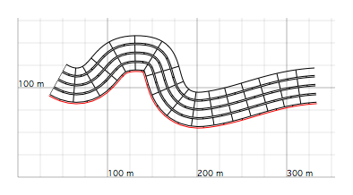
Figure 8: Pattern produced by levels 8 spacing 20 sequence (5 1). Reading the layer from top to bottom, that is, from the mother curve to the daughter curve, one recognizes the repetition of a two-term sequence made of a thick bed followed by a thinner one.

The sequence instruction can also be used to build more complex motifs, such as the following one.

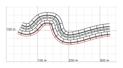
Figure 9: Pattern produced by a five-term sequence using sequence (5 1 3 2 4) levels 8 spacing 20 alternate. Since the sequence has five terms but the motif contains only eight levels, the first sequence is complete whereas the second is truncated.

In particular, sequence can be combined with graded to represent sequences that thicken or thin through time.

novertical

To suppress the transverse bars of a pattern, simply use:

  novertical

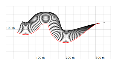
Figure 10: Pattern produced by levels 15 graded 1.6 novertical.

nohorizontal

The nohorizontal instruction suppresses all internal lines of the pattern other than the transverse ones, even if a levels or vspacing instruction has been given.

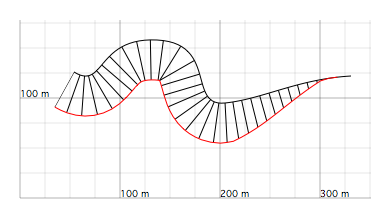
Figure 11: Pattern produced by levels 15 together with nohorizontal.

This instruction is especially useful when patterns displaying symbols are introduced later.

spacing

By default, the pattern command draws transverse bars spaced 10 metres apart. To change this spacing, use the spacing subcommand:

  spacing w

where w is the minimum distance between two bars.

Thus,

  spacing 20

produces the motif shown below, in which the transverse bars are separated by 20 metres.

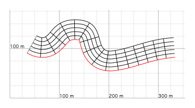
Figure 12: Pattern produced by spacing 20 levels 5.

The parameter set by spacing is an important one, because it influences other settings of the motif. It will be referred to below as the primary spacing.

alternate

A very useful instruction is alternate, which produces the conventional patterns used for limestone series, made of small staggered bricks.

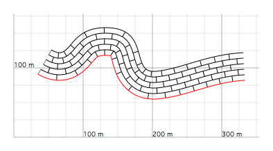
Figure 13: Pattern produced by alternate together with levels 5 spacing 20.

By default, each brick is 10 metres long. To modify this length, use the spacing subcommand.

oblique

The oblique instruction creates patterns with inclined transverse bars. Combined with alternate, it produces motifs typical of dolomitic series. In its simplest form, it is used without an argument:

  oblique

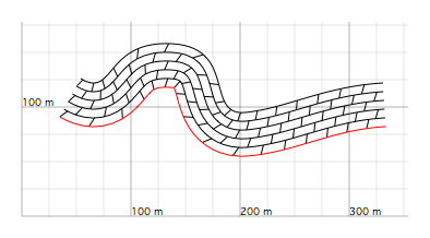
Figure 14: Pattern produced by levels 5 alternate spacing 20 oblique.

The subcommand may also be followed by a number controlling the inclination of the transverse bars:

  oblique e

where e is the longitudinal offset between the two ends of a small transverse bar.

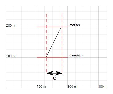
Figure 15: The obliquity e of the transverse bars.

An obliquity of 0 cancels the effect of oblique.

Obliquity also controls the direction of tilt of the bars.

By default, the obliquity is equal to one sixth of the primary spacing, and the tilt is in the same sense as the mother curve. Thus, if the mother curve is oriented from left to right, the bars tilt to the right. If the mother curve is oriented from right to left, they tilt to the left.

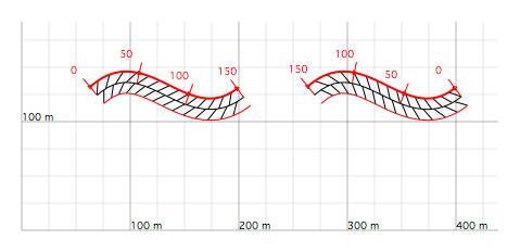
Figure 16: The direction of tilt of oblique bars is controlled by the mother curve. The two layers above were drawn with the same instructions, offset 20 pattern levels 2 oblique 8. Only the orientation of the mother curve changes. The graduations of the mother curves are displayed with graduate. On the left, the mother curve runs from left to right, so the bars tilt to the right. On the right, the mother curve runs from right to left, so the bars tilt to the left.

With a negative obliquity, the tilt of the oblique bars is opposite to the orientation of the mother curve.

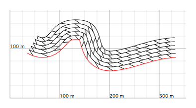
Figure 17: Pattern produced by a negative obliquity with levels 5 spacing 20 oblique -10. The mother curve is oriented from left to right.

double

The double instruction duplicates the transverse bars.

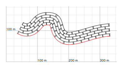
Figure 18: Pattern produced by levels 5 alternate spacing 20 double.

By default, the two parallel bars are separated by 2 metres. This distance can be modified with the spacing2 subcommand.

period

The period instruction multiplies the transverse bars. Its syntax is:

  period n

where n indicates the number of bars in each group.

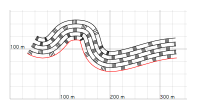
Figure 19: Pattern produced by levels 5 alternate spacing 20 period 4.

By default, the bars within each group are spaced 2 metres apart. This spacing can be modified with spacing2.

A command period 2 is equivalent to a simple double instruction.

spacing2

The spacing2 subcommand controls the spacing between transverse bars within the bar groups created by double or period. Its syntax is:

  spacing2 e

where e measures the spacing between bars inside each group. This will be referred to as the secondary spacing, in contrast with the primary spacing defined by spacing.

In what follows, let s1 denote the primary spacing, given by spacing, and s2 the secondary spacing.

When the pattern is not alternating, the bars within a given group are separated by s2, whereas s1 separates neighbouring bars belonging to different groups.

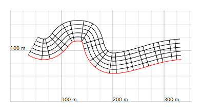
Figure 20: Pattern produced by levels 5 double spacing2 20. The double instruction creates pairs of bars. Each pair is separated from the next by 10 metres, while the two bars inside each pair are separated by 20 metres.

When the pattern is alternating, the calculation of distances is slightly more complex.

• the spacing between two neighbouring bars within the same group is s2,
• the spacing between two neighbouring bars belonging to different groups is s2 + 2 s1.

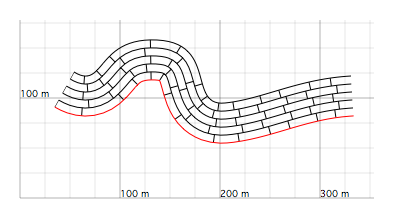
Figure 21: Pattern produced by levels 5 double spacing2 20 alternate. The motif consists of two types of bricks: some 20 metres long, equal to s2, and others 40 metres long, equal to s2 + 2 s1 = 20 + 2 × 10.

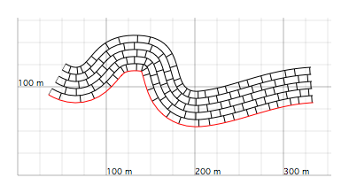
Figure 22: Pattern produced by levels 5 double spacing 6 spacing2 10. The motif is composed of two types of bricks: the smaller ones are 10 metres long, equal to s2, and the larger ones 22 metres long, equal to s2 + 2 s1.

For an alternating pattern also using period, and noting n the value supplied to period, the resulting bricks have:

• length s2, for those bounded by two bars belonging to the same group,
• length (n - 1) × s2 + 2 s1, for those trapped between bars belonging to two different groups.

It is also possible to use a primary spacing s1 equal to zero, with spacing 0, to create special motifs.

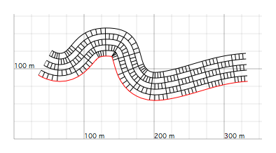
Figure 23: Pattern produced by levels 5 spacing 0 spacing2 5 alternate period 5. The small bricks are 5 metres long, equal to s2, and the larger ones are 20 metres long, equal to (n - 1) × s2.

The combination of alternate, double, period, spacing, and spacing2 makes it possible to create a very wide range of patterns.

The instructions oblique and graded can also be used in association with these subcommands, as shown below.

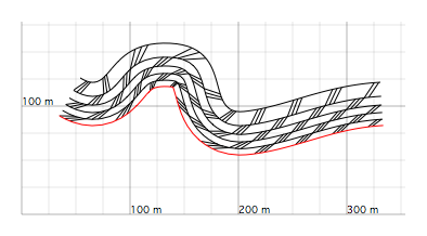
Figure 24: A relatively complex pattern produced by levels 5 alternate graded 0.7 period 3 oblique 10 spacing 20 spacing2 4.

patternoffset

The patternoffset instruction shifts the pattern laterally. Its syntax is:

  patternoffset d

where d is the lateral shift, which may be any positive or negative value. A value of 0 has no effect.

This instruction is sometimes useful for improving the visual balance of a pattern in a given layer.

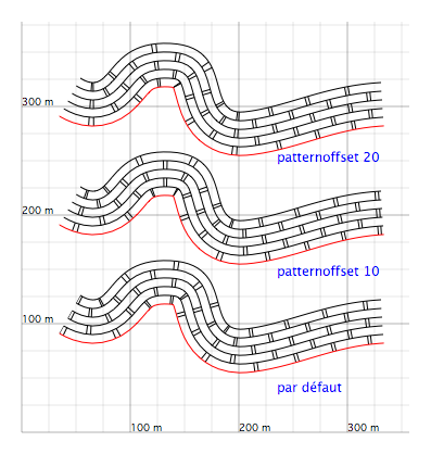
Figure 25: Effect of patternoffset for different shift values, 0 in the lower drawing, 10 in the middle one, and 20 in the upper one. A shift of 10, in the middle drawing, centers the motif more neatly around the fold hinge.

width

To control the thickness of the bars, use the width instruction:

  width f

where f is the line thickness in pixels.

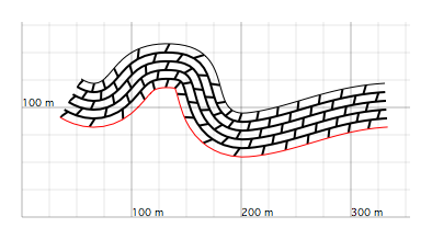
Figure 26: Pattern drawn with width 2.

dashed

The dashed subcommand draws all the bars of the pattern as dashed lines. Its syntax is described in more detail here.

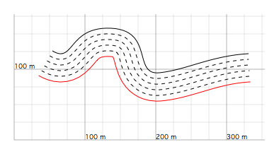
Figure 27: Pattern drawn with dashed 5 5, producing dashed median lines made of alternating solid and empty segments 5 pixels long.

dotted

The dotted instruction draws the bars of the pattern as dotted lines.

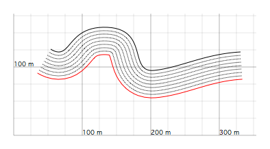
Figure 28: Pattern drawn with dotted.

base

The base instruction changes the arrangement of the lateral bars of the motif. By default, these bars are spaced by a distance defined by vspacing, 10 metres by default. This spacing is normally measured along the median line between the mother curve and the daughter curve.

With base, the spacing between the lateral bars is no longer measured along the median line, but directly along the mother curve. An illustration is given below.

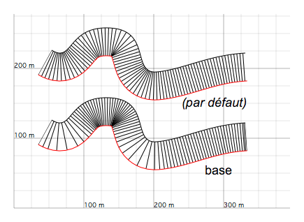
Figure 29: Comparison of patterns with lateral bars, using spacing 4, calculated without base in the upper drawing and with base in the lower drawing.

The base instruction accentuates deformations in curved areas near the daughter curve, with stronger tightening of the bars on the inner arc of folds and, conversely, looser spacing on the outer arc.