GEOD
offset
Offsetting a curve with the offset command
The offset command is one of the most important instructions in GEOD. It is this command that makes it possible to construct the offset of a curve at a given distance, and therefore to build geological layers.
Summary
- The offset command
- The offsetting operation
- Syntax
- Algorithm
- Variable-thickness layers
- Direct definition
- Using variables
- Offsets as a function of x or y
- Other options and special cases
- Highly curved lines
- Optimizing layer rendering
- Offset problems caused by too few intermediate points
- Curve closure
- Compacting layers with compact
- Simulating sedimentation with compact
- Discontinuities
- Irregular parent curves
- The method subcommand
The offset command
The offsetting operation
The offset command constructs the offset curve of another curve. This parent curve may be a Bézier curve, defined with the bezier command, a polyline defined with line, another offset curve defined with offset, or any other curve type available in GEOD. In what follows, this original curve will be referred to as the parent curve. The offset value is defined when the cross-section is built and corresponds to the thickness of the layer.
An example of an offset curve constructed from a parent curve, here a Bézier curve, is shown below.
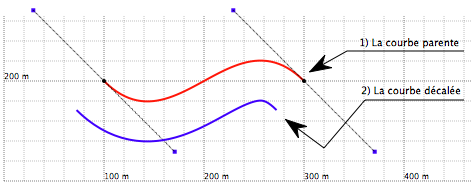
Figure 1: Construction of an offset curve, in blue, from a parent curve, a Bézier curve in red. The offset value is 40 metres. The nodes and control points of the Bézier curve are also shown.
As can be seen, these two curves form the framework used later to build a geological layer of constant thickness. The figure also shows clearly that offsetting a curve is not a simple translation. The offset curve does not have the same radii of curvature as the parent curve. Each point of the offset curve lies at the minimum distance from a point of the parent curve, and this distance is equal to the offset value. Figure 2 shows the normally invisible segments used internally by the program to calculate the offset curve. Each segment has a length equal to the layer thickness and links two homologous points, one on the parent curve and the other on the offset curve. Moreover, each of these segments is orthogonal to both the parent curve and the offset curve.
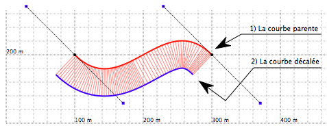
Figure 2: Calculation of the offset curve. The figure shows the segments used internally by the program. These segments connect homologous points on the parent curve and on the offset curve, and form the mesh of the geological layer.
Syntax
To offset a given curve, the parent curve, the offset command may be written in two different ways.
Full syntax:
offset name offset_value
where:
- name is the name of the parent curve, assigned earlier with the name subcommand,
- offset_value is a number specifying the offset, in other words, the layer thickness.
Example:
  bezier
      ...
      name j12
offset j12 40
Simplified syntax:
offset offset_value
In this shorter form, the parent curve is defined implicitly: it is simply the curve defined immediately before the offset instruction.
The previous example could therefore be rewritten as:
offset 40
Two remarks should be made here.
- The offset value may be either positive or negative, although a thickness is of course always a positive quantity in geological terms.
- In the full syntax, the parent curve may be defined anywhere in the script, before or after the offset instruction, or even in another script.
When the offset value is positive, the curve is offset below the parent curve. When the offset value is negative, it is offset above the parent curve.
In other words, if the offset command is used repeatedly with positive values, an entire sedimentary pile can be built downward, toward progressively older layers. With negative values, the opposite happens and the pile is built upward.
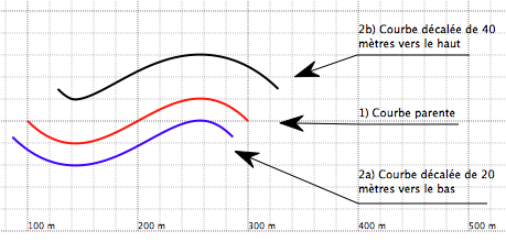
Figure 3: Offsetting upward or downward.
The offsetting algorithm
Offsetting a curve is not a simple operation. Several steps are required. To illustrate this, let us consider the calculation of the offset of a Bézier curve. The figure below shows the final result produced by GEOD.
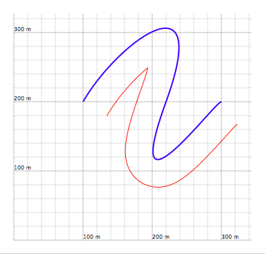
Figure 4: A Bézier curve, in blue, and its offset, in red, calculated by GEOD. The offset is 40 metres downward.
Step 1: calculation of the offset-curve points.
For each point on the parent curve, GEOD computes its homologous point on the future offset curve. As explained above, the homologous point and its generating point on the parent curve are separated by a distance equal to the offset value. At the end of this first step, a problem appears: the offset curve intersects itself in portions of low radius of curvature, for example at fold hinges. In addition, the offset curve may show an undesirable cusp at one end.
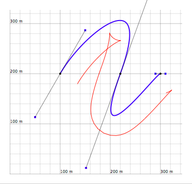
Figure 5: Step 1.
Step 2: removal of self-intersections in the offset curve.
GEOD automatically removes self-intersections in the offset curve. As shown in the figure below, this resolves the problems at fold hinges, but the cusp problem may still remain.
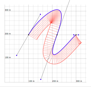
Figure 6: Step 2. Self-intersections in the offset curve have been removed, but crossings between segments linking homologous points are still visible.
Step 3: elimination of intersecting segments.
To remove these cusps, GEOD searches for all intersecting segments and suppresses them. More precisely, the program removes the points on the offset curve that generate these artefacts. It is then up to the user to complete the parent curve, possibly with extendfirst or extendlast, in order to deal with these undetermined edge effects in the rendering of offset curves.
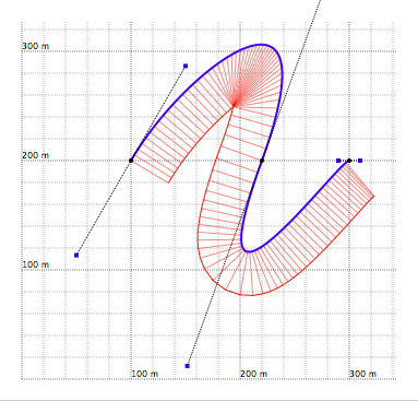
Figure 7: Step 3: elimination of homologous points belonging to intersecting segments.
This part of the algorithm is especially useful when the parent curve includes steep segments or abrupt changes in dip. An illustration is given by the animation referred to in the original manual.
Step 4: insertion of points in segments that are too sparse.
When GEOD draws a curve, whether a polyline or a Bézier curve, it ensures that intermediate points are spaced at no more than 5 metres apart by default. However, neighbouring points on the offset curve may end up farther apart, especially in highly curved parts. To solve this, GEOD inserts additional intermediate points in all portions of the offset curve that are too sparse.
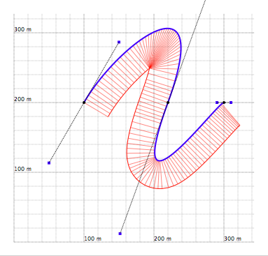
Figure 8: Step 4: densification of points in sparse parts of the offset curve. Compare this figure with Figure 7 to see the additional points, especially on the outer arc of the fold.
It is this final step of the algorithm that ensures a good rendering of offset curves, even in highly curved areas.
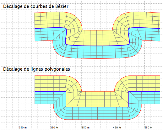
Figure 9: Offsetting L-shaped curves. The parent curve is shown in blue and has been offset both upward and downward. A critical part of the calculation is the treatment of rounded corners. This is achieved by inserting additional intermediate points.
Variable-thickness layers
GEOD can also draw layers of variable thickness, including wedge-shaped layers that locally pinch out. There are two ways to do this: either by defining the thickness variations directly in the offset instruction, or by using GEOD variables defined with the set command.
Direct definition
To construct a variable-thickness layer, GEOD uses the curvilinear coordinate scale of the parent curve. The offset values are no longer constant, but vary as a function of the curvilinear coordinate u. In GEOD, these offset variations are represented by piecewise linear functions with the following syntax:
  offset
      lineName
      (
      value1 at u1
      value2 at u2
      ...
      valuen at un
      )
GEOD uses the pairs u1-value1, u2-value2, ..., un-valuen to constrain the offset values at successive curvilinear coordinates. For any curvilinear coordinate u, the program calculates the offset value by linear interpolation between the two surrounding points.
Use the graduate instruction on the parent curve to display curvilinear coordinates temporarily.
For example, the following code produces the layer shown in Figure 10:
  line
      100 100
      dir 0 500
      graduate above
      color black
  offset
      ( 20 at 50, 50 at 100, 50 at 200, 0 at 250, 0 at 275, -50 at 300, -50 at 375, 0 at 400, 0 at 450, 20 at 450 )
      color blue
pattern debug
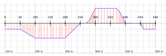
Figure 10: Variable-thickness layer. The parent curve is shown in black, with curvilinear coordinates displayed by graduate. The offset curve is shown in blue. The offset varies linearly according to the instructions entered in the script. The layer thickness may locally vanish, and may even alternate above and below the parent curve.
Using variables
Another way to construct a variable-thickness layer is to use the set command, which defines variables in GEOD.
This technique is somewhat heavier, but it may be useful when the cross-section contains several layers sharing the same geometry.
The thickness variation is defined using the same syntax as above, but now through a variable defined with set:
  set d to var
      ( 0 at 0, 20 at 50, 20 at 100, 0 at 150 )
In this example, the information describing the thickness variation is stored in a variable named d. This is a spatial variable, as indicated by the expression to var.
To offset a curve, one then writes:
offset lineName with variableName
where:
- lineName is the name of the parent curve to offset. This argument is optional.
- variableName is the name of the variable declared with set ... to var.
The example below illustrates the construction of a sedimentary accumulation made of stacked lenses. The initial parent curve is the topographic profile. All the other curves are produced by instructions of the form:
offset with d
Each offset curve then serves as the parent curve for the next offset instruction. To prevent the lenses from always overlapping at the same location, and to shift them alternately left and right, the u0 instruction is used. This instruction makes it possible to change the origin of the curvilinear coordinates.
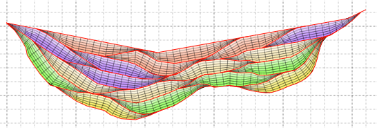
Figure 11: Accumulation of sedimentary lenses produced by successive curve offsets, where the offset values are functions of the curvilinear coordinates of the parent curves.
Offsets as a function of x or y
By default, GEOD uses the curvilinear coordinate u of the parent curve to calculate the thickness of the layer. It is also possible to specify thickness as a function of the horizontal coordinate x or the vertical coordinate y.
To offset as a function of x, write:
offset lineName ( ... ) as x
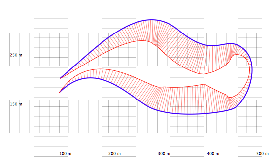
Figure 12: Example of an offset defined as a function of x. The parent curve, in blue, is a Bézier curve.
To offset as a function of y, write:
offset lineName ( ... ) as y
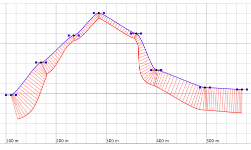
Figure 13: Example of an offset defined as a function of y. The parent curve, in blue, is a Bézier curve.
Options and special cases
Highly curved lines
As explained above, GEOD inserts extra points in strongly curved parts of the offset curve. It does so only up to a certain limit. Beyond a threshold, GEOD simulates an opening fracture, because geological layers are not infinitely ductile.
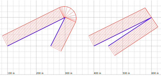
Figure 14: The blue line is the parent curve and the red line is the offset curve. On the left, the offset is strongly curved but remains continuous. On the right, the curvature is even stronger and produces a clear break.
Optimizing layer rendering
To construct a curve, GEOD inserts a number of intermediate points between two nodes of a polyline or a Bézier curve. These intermediate points are then used by the offset command to construct a layer. Their number affects both the computation speed and the quality of the rendering.
For a polyline, defined with line, or a Bézier curve, defined with bezier, the number of intermediate points is proportional to the distance between two nodes. By default, the program inserts one intermediate point approximately every 5 metres, a value that can be modified with seglen. In all cases, the number of inserted segments is limited to a maximum of 50, a value that can be modified with segnb.
The user can act in three different ways to optimize the rendering of offset curves built from Bézier curves.
First method: use segnb.
This subcommand reduces the number of intermediate points inserted between two nodes of a Bézier curve.
  bezier ...
      segnb 10
This tells GEOD to use at most 10 intermediate points instead of 50.
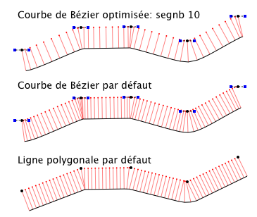
Figure 15: Optimizing the rendering of offset curves. The parent curves are shown in black and the offset curves are displayed with the dot option so that intermediate points are visible. The homologous segments are highlighted with pattern debug. The bottom drawing uses a polyline, the middle drawing a Bézier curve with too many intermediate points, and the top drawing the same Bézier curve but with segnb 10, which brings the number of intermediate points back to a reasonable level.
Second method: use resolution.
resolution 10
This reduces the number of intermediate points in both the parent curve and the offset curve.
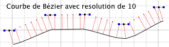
Figure 16: Reduction in the number of intermediate points in a Bézier curve using resolution 10.
Be careful: the resolution command applies to all curves in the drawing, whereas segnb and seglen affect only the parent Bézier curve.
Third method: use the minseglen and maxseglen subcommands specific to offset.
minseglen sets the minimum separation distance between intermediate points on the parent curve that will be used to calculate the offset curve.
minseglen 10
This means that GEOD will calculate the offset of a point on the parent curve only if it is at least 10 metres away from the previous intermediate point.
This avoids taking too many points into account, especially in very dense portions of the parent curve.
By default, the value controlled by minseglen is 1 metre, corresponding to the global value fixed by resolution.
In contrast, maxseglen controls the maximum separation distance between intermediate points on the offset curve.
maxseglen 50
This tells GEOD to insert additional points in the offset curve, and in the parent curve, only if two adjacent intermediate points on the offset curve are at least 50 metres apart.
By default, the value set by maxseglen is twice 5 metres, that is, 10 metres.
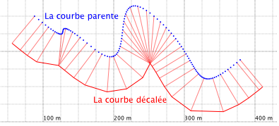
Figure 17: The minseglen and maxseglen instructions applied to an offset curve, here minseglen 10 and maxseglen 50.
Choosing a high value for maxseglen, for example maxseglen 1000, effectively disables the insertion of extra points in sparse portions of the offset curve.
Offset problems caused by too few intermediate points
Offset problems may also occur when the parent curve does not contain enough intermediate points. This situation can be diagnosed when the segments linking homologous points are no longer orthogonal to the curves. The problem can be solved by adding more nodes to the parent curve, or by densifying the intermediate points using segnb or resolution.
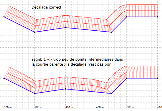
Figure 18: Curve offsetting. The parent curve, in blue, is a Bézier curve. The homologous segments are highlighted with pattern debug. In the lower case, the Bézier curve lacks enough intermediate points and the offset cannot be computed correctly. In the upper case, the rendering is correct because the number of intermediate points is sufficient.
Curve closure
The offsetting algorithm described above cannot handle offset curves that close back onto themselves, as may happen in very tight folds.
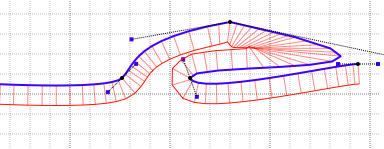
Figure 19: Initial stage before closure. The blue curve is the parent curve and the red curve is the offset curve.
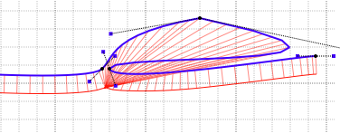
Figure 20: Stage after closure. GEOD can no longer calculate the offset curve correctly.
Simulating compaction with the compact subcommand
The offset command includes a subcommand called compact, which is useful for creating animations in GEOD. This subcommand makes the offset value, in other words the layer thickness, depend on time.
  offset ...
      compact degreeOfCompaction
where degreeOfCompaction is a variable with values between 0 and 1. The effective offset is obtained by multiplying the nominal offset value by (1 - degreeOfCompaction).
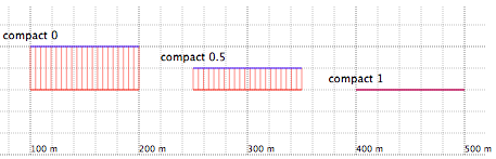
Figure 21: The compact subcommand used to compact a sedimentary formation. The parent curve is shown in blue.
degreeOfCompaction can be written as a time-dependent variable. For example, to simulate a layer losing 80% of its thickness in one second, write:
  offset ...
      compact (
          0 at 0,
          0.80 at 1
      )
One may also use a time-dependent variable defined with the set command as follows:
  offset ...
      compact with c0
  set c0 to time
      ( 0 at 0, 0.8 at 1 )
This approach is especially useful for animations of progressive burial and compaction.
Simulating sedimentation with compact
The compact instruction can also be used to simulate the progressive accumulation of sediments. In that case, one starts from a compaction degree of 1 and lets it decrease to 0.
  offset ...
      compact ( 1 at 0, 0 at 5 )
This makes it possible to animate the filling of a sedimentary basin.
Discontinuities
The offset command can handle discontinuities created in Bézier curves or polylines with the gap subcommand. The resulting offset curve will itself contain discontinuities.
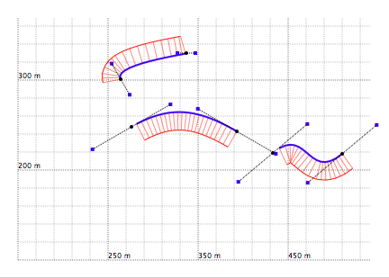
Figure 22: Discontinuities in the offset curve produced by gap instructions in the definition of the parent curve, whether it is a polyline or a Bézier curve.
Irregular parent curves
Parent curves with an irregular trace, for example bayonet-like, zigzag, or step-like paths, are generally handled correctly by GEOD. However, when such layers are examined closely, especially in debug mode with pattern debug, one may sometimes observe intersections among the homologous segments.
We have seen that GEOD normally removes such intersections during the third step of the offsetting algorithm. However, these new intersections may in fact appear later, during the fourth step, when additional points are reinserted into sparse portions of the curve.
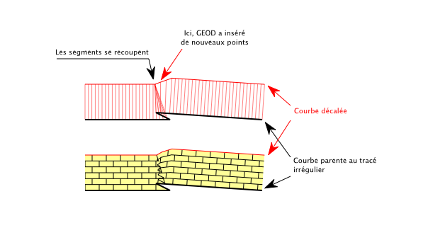
Figure 23: Intersections of homologous segments. The upper drawing shows debug rendering with pattern debug, and the lower drawing shows the final rendering with a lithological pattern applied.
Although this type of problem slightly perturbs the final lithological rendering, it often gives a rather realistic impression of a faulted zone.
The method subcommand
For correct rendering of layers, GEOD removes intersections among the homologous segments, as described in the paragraph on the offsetting algorithm. In its current version, GEOD provides two different algorithms for handling these segment intersections. This option is accessible with the method subcommand.
By default, GEOD uses the first algorithm.
method flag
where flag is an integer between 0 and 2.
- if flag = 0, GEOD disables the treatment of intersecting segments. This speeds up rendering, but may leave artefacts and spurious lines.
- if flag = 1, GEOD applies the default algorithm.
- if flag = 2, an alternative method is used.
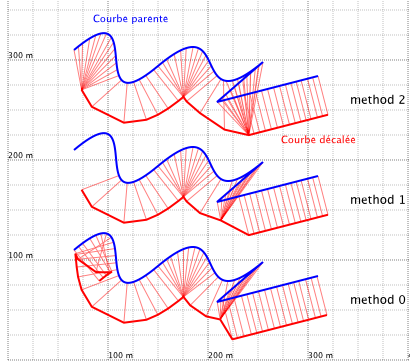
Figure 24: Different algorithms for handling segment intersections with the method subcommand. The parent curve is shown in blue, the offset curve in red, and the homologous segments are highlighted with pattern debug. In these examples, the insertion of extra points into sparse portions has been disabled.
The two active methods differ in principle.
- For method 1, the program first counts the number of intersections for each segment. It then identifies the segment responsible for the largest number of intersections and removes it, more precisely by deleting the corresponding point on the offset curve. The homologous point on the parent curve is then left without counterpart. The program repeats this process until all intersecting segments are removed.
- For method 2, the program searches for all intersecting segments, regardless of the number of crossings. As soon as an intersection is found, the point at the end of the segment on the offset curve is reassigned the coordinates of the nearest point belonging to a non-intersecting segment.
This has consequences for performance and behaviour.
- Method 2 is faster, because a single pass along the offset curve is sufficient, whereas method 1 must iterate until all intersecting segments have disappeared.
- Method 1 destroys intermediate points, whereas method 2 merely changes their position.
The method instruction is a subcommand of individual offset curves. If the same method is to be applied to all offset curves in the cross-section, it must otherwise be repeated for each one. For this reason, GEOD also provides a global command called offsetmethod:
offsetmethod flag
where flag has the same meaning as for method.
This command may be inserted anywhere in the script, and it applies to all offset curves.