GEOD

image (2)

Reconstructing a digital elevation model with the image command

The image command may also be used to reconstruct a digital elevation model by digitizing contour lines from a scanned map in a GEOD window.

Summary

• Reconstructing a digital elevation model from contour lines digitized on a scanned map
  • Step 1: creating an empty DEM
  • Step 2: the plane instruction
  • Step 3: defining spot heights with zpoint
  • Step 4: interpolating elevations with voronoi
  • Step 5: defining contour lines with zline
  • Step 6: interpolating elevations with MNT
  • Step 7: saving the DEM with export
• Other subsidiary functions that may be useful for DEM construction
  • The tilt instruction
  • The zellipse instruction
  • The noise instruction
  • The resize instruction

  Reconstructing a digital elevation model from contour lines digitized on a scanned map

This section illustrates various GEOD functions that make it possible to recreate a complete digital elevation model from elevation data.

Step 1: creating an empty DEM

The first step is to define a point grid of given dimensions with the image command. As explained above, one may write in the script window:

  image ""
      width 400
      height 300

but this time the `image` command is not followed by the name of a DEM file to load. In this case, or when the name refers to a nonexistent file, GEOD reconstructs a DEM from the script instructions. In the present example, GEOD fills a rectangular area on the screen, 400 metres wide and 300 metres high, with black pixels corresponding by default to an elevation of 0 metre.

Figure 1 : Creation of a DEM over an area measuring 400 m by 300 m.

×

Step 2: the plane instruction

Once the DEM dimensions are fixed, the elevations still have to be defined at each point of the grid. For this, the simplest instruction is the plane subcommand, which assigns the same elevation value to all points of the DEM. For example, to specify an altitude of 100 metres, which is the default value, one writes:

  plane 100

This instruction is placed after the image command, either directly or after other instructions such as width, height, x, or y.

Figure 2 : Defining a default elevation on the DEM with a plane instruction.

The plane instruction may also be used to erase all elevation values. For this, one writes:

  plane erase

Step 3: defining spot heights with zpoint

Spot heights are defined with the zpoint instruction. This instruction requires three arguments, namely the x and y coordinates of the point and its elevation z. There are four different ways to define these arguments.

• The point may be defined by its coordinates in the DEM reference system. For example:

  zpoint 100 200 250

defines a spot-height point at the grid node with coordinates x = 100 and y = 200. The point x = 0 and y = 0 lies at the lower-left corner of the DEM. The value of x must lie between 0 and the grid width minus 1, and the value of y must lie between 0 and the grid height minus 1. The third argument, here 250, gives the elevation of the point.

• The point may also be defined by its coordinates in the GEOD figure reference system. In that case, the coordinate values must be preceded respectively by the keywords x and y. Thus:

  zpoint x 200 y 100 150

places a spot-height point of elevation 150 at coordinates x = 200 and y = 100 of the GEOD figure.

With this method, care must be taken not to move the DEM inadvertently by x and or y instructions within the GEOD figure, because points defined in this way remain fixed in the GEOD window.

• A third method uses a user-defined reference system on the DEM. The coordinate values must then be preceded by the keywords xref and yref. For example:

  zpoint xref 300 yref 200 200

defines an elevation z = 200 at the point with coordinates x = 300 and y = 200.

• Finally, a fourth technique consists in using a point defined by a point command, as in the following example:

  zpoint p 220

where p is the name of a point defined by a point command, and 220 is the elevation of the point:

  point x 200 y 200
      name p
      hidden

To hide the point, one adds, as above, a hidden instruction.

The set of instructions above produces the DEM illustrated in figure 3. At this stage, elevations are defined only at four points, visible as four white pixels on a black background.

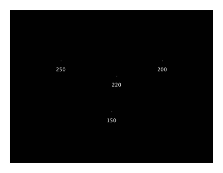
Figure 3 : Definition of four spot-height points on a DEM. These points are barely visible as four light-coloured pixels. The numbers indicate their elevations.

Step 4: interpolating elevations with voronoi

The spot-height points defined previously are sufficient to build a first version of the DEM by the Voronoi method. The basic idea is to assign to every node of the grid the elevation of the nearest spot-height point.

In fact, for efficiency reasons, the algorithm implemented in GEOD does not follow this principle strictly, although it remains close to it. It is inspired by crystal-growth mechanisms in nature. Each spot-height point serves as a nucleation seed from which elevations are determined progressively in neighbouring pixels. In general, as expected, a pixel will indeed be coloured according to the nearest spot-height point. But the algorithm also tends to overestimate the influence zone of a point along certain preferred directions, namely N-S, E-W, NW-SE, and NE-SW, because of the square grid geometry.

Although the result is not exactly what a true Voronoi algorithm would produce, the name has been retained. The DEM obtained is composed of a series of plateaus centred on the spot-height points.

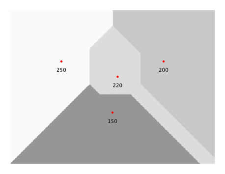
Figure 4 : A first DEM constructed by the Voronoi method from the four spot-height points of figure 3.

Step 5: defining contour lines with zline

Contour lines allow the DEM to be constrained more effectively. For this purpose, one uses the zline instruction. This is done in two stages.

• First, the contour lines are drawn with line or bezier commands. These curves should also be named with a name instruction.

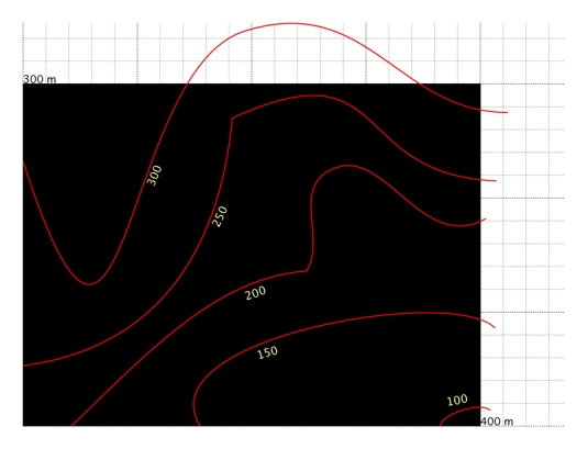
Figure 5 : Drawing contour lines with bezier commands on the black background of the DEM.

• Next, these curves are associated with the DEM by means of the zline instruction. For each contour line, one writes a zline instruction in the body of the image command, as follows:

  image a0.txt
      ...
      zline name altitude

where name must be replaced by the name of the curve drawn with a line or bezier command, and altitude by the elevation in metres of the contour line.

With this instruction, GEOD replaces all pixels covered by the contour line by assigning them an elevation value.

Figure 6 shows the result after the Bézier curves have been hidden with a hidden instruction.

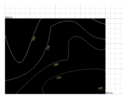
Figure 6 : Contour lines drawn onto the DEM with zline. The brightness of the lines depends on elevation.

Once the contour lines have been incorporated into the DEM, the elevations between them still have to be interpolated. As explained above, two methods are available.

• The first uses the voronoi instruction. It gives a rudimentary but fast representation of the DEM in the form of a series of steps.

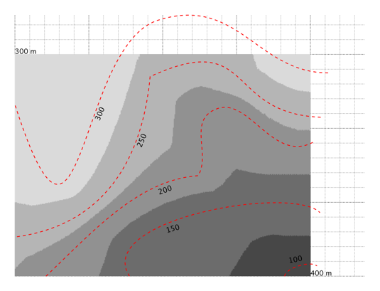
Figure 7 : DEM obtained with the voronoi instruction.

• The second method is described in the following paragraph.

Step 6: interpolating elevations with MNT

The MNT instruction smooths the elevations between contour lines. The resulting DEM is much more realistic than the one obtained with the voronoi instruction.

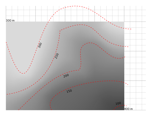
Figure 8 : DEM obtained with the MNT instruction.

Step 7: saving the DEM with export

To store the DEM once created, one uses the export instruction. The elevations are then saved in a data file for later reuse. The syntax is simple:

  export "..."

where ... inside quotation marks must be replaced by the path of the file, or simply by its name if the file is to be saved in the same folder as the script currently being edited.

Two file formats are available:

• The data may be saved in an ASCII format readable by GEOD. In that case, the file name must end with the extension .txt.

Example:

  export "myMNT.txt"

The advantage of the ASCII format is that this type of file may also be used by other DEM-processing software. However, the resulting files are larger and their reading by GEOD takes longer.

• Alternatively, the data may be saved in a binary format, also directly readable by GEOD. The file name must then end with the suffix .dem.

Example:

  export "myMNT.dem"

These binary files have the advantage of being more compact and quicker to read. However, their format is not recognised by software other than GEOD.

Remark:

The different instructions associated with the image command, such as zpoint, zline, voronoi, MNT, export, and others, are executed sequentially, that is, in the order in which they appear in the script. Therefore, the export instruction should be placed last in order to save the final version of the DEM. Otherwise, an intermediate version or even an empty DEM may be saved.

Other subsidiary functions that may be useful for DEM construction

The tilt instruction

The tilt instruction is used to construct the DEM of an inclined plane. It follows the same syntax as zpoint, but with additional parameters.

  tilt x y
      azimuth dip

or

  tilt x x y y
      azimuth dip

or

  tilt xref x yref y
      azimuth dip

See this paragraph to understand the differences between these syntactic forms.

The additional parameters azimuth and dip give respectively the azimuth of a horizontal line of the plane and the dip of the plane.

The tilt command associated with a zlap instruction makes it possible to display colour gradients.

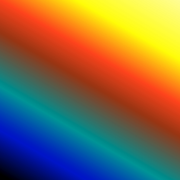
Figure 9 : The tilt instruction used to display gradients.

The zellipse instruction

The zellipse instruction is used to draw an elliptical zone of constant elevation on the DEM. The syntax is:

  zellipse x x y y
      z
      r1
      r2
      angle

where z is the elevation of the elliptical zone, r1 and r2 are the radii of the ellipse, and angle measures the inclination of the ellipse relative to the horizontal axis of the DEM.

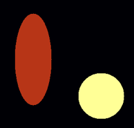
Figure 10 : The zellipse instruction used to draw ellipses and circles.

The noise instruction

The noise instruction is used to add noise to the DEM, giving it a more realistic and less artificial appearance. Its syntax is:

  noise type sigma

where type sets the kind of noise, with 0 for uniform noise and 1 for Gaussian noise, and sigma sets the noise level.

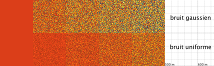
Figure 11 : Adding noise to images with different noise instructions.

The resize instruction

The resize command is used to resample an image. Its syntax is:

  resize zoom type

where zoom is a number giving the reduction or enlargement factor of the image, and type specifies the method used to compute interpolated pixels. Three methods are available:

• type = 0: the interpolated pixel takes the value of the nearest non-interpolated pixel.
• type = 1: the interpolated pixel is obtained by linear interpolation from the nearest pixels.
• type = 2: the interpolated pixel is computed by cubic interpolation from the nearest pixels.

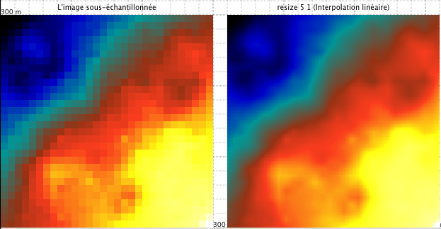
Figure 12 : Effect of the resize command. On the left, resize has been used to downsample an image. On the right, the image on the left has been resampled again, also using resize.