GEOD

image (1)

Displaying an image with the image command

The image command is used to display an image, for example a scanned extract of the geological map next to the cross-section line. This command is also able to load topographic data from a digital elevation model and display it as a grayscale image or as a false-colour image.

Summary

Displaying an image
The image command

To insert an image into a GEOD figure, one uses the image command followed by the file path enclosed in double quotation marks:

  image "..."

where ... must be replaced by the path of the graphic file.

The file path may be specified either as an absolute path:

  image "Macintosh HD/Users/regis/Documents/geod/data/image1.pdf"

or as a relative path from the folder containing the GEOD script currently being edited:

  image "../data/image1.pdf"

In this second case, the script must have been saved beforehand before pressing the `Enter` key, otherwise the image will not be displayed in the preview window.

The image command is able to load the main standard image formats, including PDF, JPEG, PNG, GIF, BMP, and others.

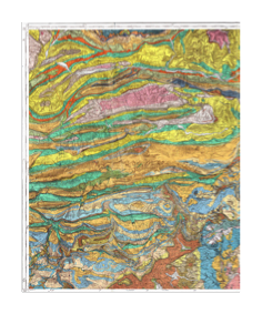
Figure 1 : Display of a scanned map with an image command. The example shown is an extract of the Nice geological map at 1:80,000 scale, saved in PDF format.

It should also be noted that:

several images may be displayed simultaneously in the same figure.
to speed up the updating of the figure during the construction of the cross-section or structural sketch, GEOD uses a cache memory for figure display. Even when the scanned map is rather large, refreshing remains fast, which makes interactive work reasonably comfortable.

Sizing the image with width and height

To control the display size of an image, one uses one of the subcommands width or height. For example:

  width 300

sets the image width to 300 pixels, that is, 300 metres with the default GEOD settings. In order to preserve the aspect ratio of the image, GEOD modifies the height proportionally.

Instead of width, one may use the height subcommand to set the height directly, for example to 200 pixels:

  height 200

If both subcommands are used simultaneously, the width instruction takes precedence over height, in order to preserve the proportions of the image.

Positioning the image with x and y

To position the image within the figure, one uses the x and or y instructions. For example:

  image "..."
      x 100 y 50

places the lower-left corner of the image at the point with coordinates x = 100 m and y = 50 m.

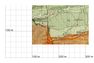
Figure 2 : The instruction x 100 y 50 used to move the image.

Loading a digital elevation model

The image command in GEOD also provides access to several basic functions for handling digital elevation model data.

ASCII DEM files

A digital elevation model may be loaded with the image command. In this case, the data file must be formatted as an ASCII file and must end with the extension `.txt`. For example, the instruction

  image "sthelens.txt"

displays the DEM of Mount Saint Helens stored in the file `sthelens.txt`.

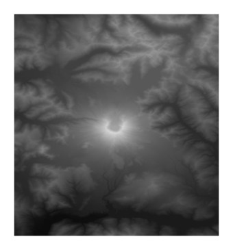
Figure 3 : Digital elevation model of Mount Saint Helens.

The DEM file format is simple. It contains elevation values measured on a rectangular grid of regularly spaced points.

the first value, nx, is the number of points in each row of the grid, that is, the number of points along the east-west direction.
the second value, ny, is the number of points in each column of the grid, that is, the number of points along the north-south direction.
the remainder of the file consists of nx × ny elevation values, expressed in metres, measured point by point from the upper-left corner of the DEM to the lower-right corner.

Note that by clicking on any point of the DEM, GEOD displays the point coordinates together with its elevation in the text area located at the bottom of the document window. For each x and y coordinate, GEOD displays two values:

the first is the offset in pixels relative to the lower-left corner.
the second, shown in parentheses, gives the offset in metres relative to the origin.

Finally, the elevation z, expressed in metres, is displayed at the end of the line.

Figure 4 : Text area displayed at the bottom of the document window. When clicking on a DEM image, GEOD displays information about the selected point.

Binary DEM files

GEOD is also able to read DEM files in binary format. These data files can no longer be examined with a text editor, but they have the advantage of being loaded very quickly into memory. These files use the extension `.dem`. Note that these files are created by GEOD itself, as explained in the section on the export instruction, and therefore follow a format specific to GEOD.

  image "mnt1.dem"

Encoding elevations with zmin and zmax

The DEM is displayed in 255 grayscale levels. By default, elevations of 0 metres are represented by black pixels, while elevations of 255 metres are represented by white pixels. In most cases, it is necessary to modify these default settings, because all information for elevations below 0 metres and above 255 metres is otherwise lost. For this purpose, the zmin and zmax instructions are used to change the image encoding. In the example above, assuming elevations range between 50 m and 3000 m, one adds the following instructions:

  zmin 50
  zmax 3000

Time-dependent zmin and zmax parameters may also be used with tables. For example:

  zmin (50 at 0, 100 at 2)
  zmax (3000 at 0, 2000 at 3)

False-colour display with zmap and zlap

It is possible to produce a false-colour view of the DEM with the zmap and zlap instructions.

zmap colours the DEM by assigning a uniform colour to each elevation range. Several predefined colour tables are available. In the example below, the colour table geo is used. This table uses five different colours, from blue to cyan, green, yellow, and red in the direction of increasing elevations. The elevation ranges depend on the minimum and maximum altitude values specified by the zmin and zmax instructions.

  image "sthelens.txt"
      zmap geo

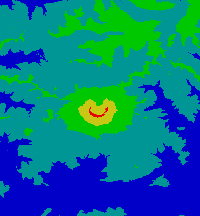
Figure 5 : False-colour display produced with zmap.

By contrast, the zlap instruction colours the DEM with gradual false-colour gradients.

  image "sthelens.txt"
      zlap geo

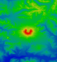
Figure 6 : False-colour display produced with zlap.

Other colour tables are also available, identified by the following names: red, green, blue, cyan, yellow, magenta, copper, gold, hot, and cold.

One may also define a custom colour table by using the syntax:

  image "sthelens.txt"
      zmap (
          colorName at ...,
          colorName at ...,
          red green blue at ...
      )

where colorName must be replaced by a colour name such as red, green, blue, cyan, yellow, magenta, black, or white, and where the ... must be replaced by an elevation value. Colours may also be specified by their red, green, and blue components, expressed as values between 0 and 255. For example, one may write:

  image "sthelens.txt"
      zmap (
          red at 0,
          blue at 1000,
          200 100 40 at 2000
      )

Displaying interference fringes with interfero

The interfero instruction makes it possible to simulate DEM relief by means of interference bands.

  interfero

The bands are calculated from the zmin and zmax parameters. By modifying these values, one may adjust the width of the bands. The false colours themselves are specified with a zmap or zlap instruction.

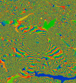
Figure 7 : DEM of Mount Saint Helens represented by interference bands. Horizontal surfaces are clearly highlighted by areas of uniform colour.

Automatically adjusting image dynamics with automatic

Knowledge of the minimum and maximum elevations is necessary for the zlap and zmap instructions in order for the image to be displayed optimally. One may either provide this information manually with the zmin and zmax instructions, or use the automatic instruction:

  automatic

Specifying geographic coordinates with reference

The geographic coordinates of the DEM are not stored in ASCII or binary files. They must therefore be specified in the script. This information is transmitted to GEOD by means of the reference instruction. Its syntax is:

  reference xmin ymin xmax ymax

where xmin ymin xmax ymax indicate respectively the real geographic (x, y) coordinates in metres of the lower-left point, that is, the south-west corner, and of the upper-right point, that is, the north-east corner, of the DEM.

The reference instruction is especially useful for establishing topographic profiles.