GEOD

bezier

Bézier curves

Bézier curves are parametric curves commonly used in drawing software. They make it possible to construct smooth and sinuous curves rapidly from a small number of points, called nodes or nodal points.

Summary

Construction
Basic syntax
Break points
Polarity
Other useful instructions for Bézier curves
The name subcommand
The extendfirst and extendlast subcommands
The hextendfirst and hextendlast subcommands
The gap subcommand
The control subcommand
The graduate subcommand
The dot subcommand
The segnb and seglen subcommands
The resolution command
The tie subcommand
The dir subcommand
The fix subcommand
The rel subcommand
Other instructions shared with the line command

Construction

Basic syntax

A Bézier curve is defined with the bezier command, followed by the definition of its nodes.

Each node, or nodal point, is defined by:

its coordinates, using the x and y subcommands. x defines the horizontal position of the point, and y its elevation.
its slope, that is, the angle of the tangent to the curve relative to the horizontal. This angle, called dip in geology, is measured in degrees clockwise and is defined by the slope subcommand. Slope information may be omitted, and by default the slope of a node is 0.
its range, which defines the zone of influence of the node on the Bézier curve. The range is defined with the range subcommand. By default, a point has a range of 10 metres on both sides.

Syntax for coordinates:

  x value
  y value

Syntax for slope:

  slope value

Syntax for range:

  range value

Here is an example of a Bézier curve definition with two nodes.

  bezier
      x 100 y 100
      slope -10
      range 50

      x 300 y 220
      slope 45
      range 200

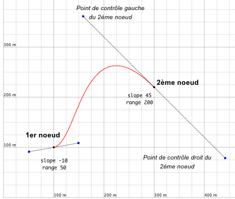
Figure 1: Bézier curve constructed with the instructions above. In this figure, the nodes and their tangents are shown. They are normally hidden and were displayed here using the control subcommand.

In the figure above, the nodes are highlighted by the control subcommand and are represented by small black points. The range and slope are visualized by a dashed segment tangent to the Bézier curve at the node. The ends of this segment are the control points of the node and are drawn as small blue squares. The range is the distance between the node and its control points.

A Bézier curve can also be constructed from a single node. In that case, the curve consists of a single segment.

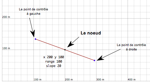
Figure 2: Bézier curve defined from a single node. The components of the curve, node, tangent, and control points, are displayed with the control subcommand.

Break points

When the curve undergoes abrupt changes in dip, it is possible to insert break points. These are nodes with different slopes and ranges on the left and right sides.

Use the leftslope and rightslope subcommands to specify the dip respectively on the left and right side of the nodal point. These subcommands follow the same syntax as slope, where value is the angle in degrees of the half-tangent relative to the horizontal. A positive value indicates that the half-tangent points downward, whereas a negative value indicates that it points upward.

  leftslope value
  rightslope value

In the same way, the leftrange and rightrange subcommands are used to assign different ranges on the left and right of the node.

  leftrange value
  rightrange value

where value is the range in metres.

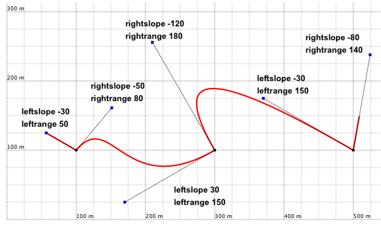
Figure 3: Illustration of leftslope, rightslope, leftrange, and rightrange used to create break points on a Bézier curve.

Polarity

Bézier curves and layer boundaries share several important properties.

Like layer boundaries, Bézier curves are drawn from coordinates and dip values. The range defined at each node also indicates the relative importance of the dip, that is, whether it is only a very local value or not.
As for any geological boundary, the different points of a Bézier curve also have a polarity. In other words, where is the top, and where is the base? Is the geological layer in normal or overturned position?

The figure below shows four Bézier curves, drawn as thick dark blue lines, which were used to construct two layers. These four Bézier curves were defined in the same way, with the same nodes, the same slopes, and the same ranges. The only difference concerns the polarity of the points. This shows clearly that a simple inversion of polarity at one point can modify the entire overall structure.

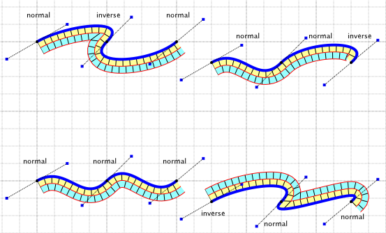
Figure 4: Polarity of Bézier curve nodes. The dark blue line is the Bézier curve. The cyan layer is older than the yellow layer.

There are three ways to define an inverse polarity for a node.

The first way is to specify a slope between 90° and 180°, or between -90° and -180°.
The second way is to insert the inverse instruction in the definition of the node.

  bezier
      x ...
      y ...
      slope ...
      range ...
      inverse

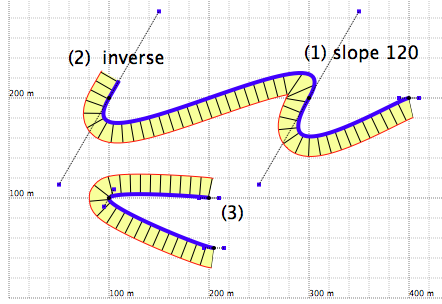
The third solution is sometimes to do nothing at all. GEOD is able to detect overturned layers produced by certain geometric configurations.

Figure 5: How to construct an overturned layer. In blue, a Bézier curve is drawn, representing the roof of a layer shown in yellow, overturned locally using the techniques described above.

Other instructions

Most of the subcommands presented earlier for the line command can also be used with Bézier curves. They are recalled here for convenience.

The name instruction

This instruction assigns a name to the curve. See also the corresponding paragraph.

  name aName

The extendfirst and extendlast instructions

These subcommands extrapolate the curve at its ends. See the corresponding paragraph.

  extendfirst 100

  extendlast 100

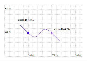
Figure 6: The extendfirst and extendlast instructions applied to a Bézier curve. The initial ends of the Bézier curve are marked with symbols.

The hextendfirst and hextendlast instructions

These work in the same way, except that the extrapolation is performed in a horizontal direction. See the corresponding paragraph.

  hextendfirst 100

  hextendlast 100

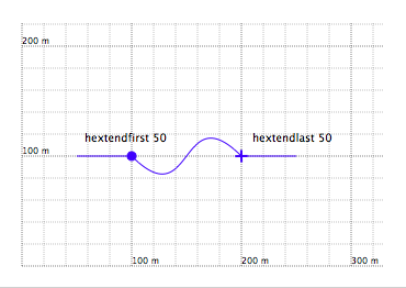
Figure 7: The hextendfirst and hextendlast instructions used to extrapolate a Bézier curve horizontally.

The gap instruction

gap allows a Bézier curve to be built in several separate pieces. Simply insert this instruction between two node definitions of the Bézier curve. See the corresponding paragraph.

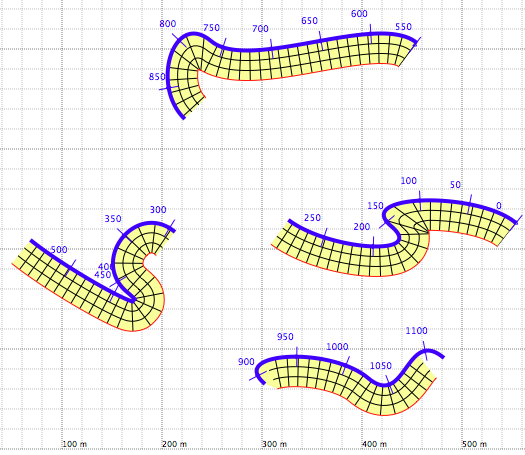
Figure 8: The gap instruction used to split a Bézier curve into several pieces. The blue segments above all belong to a single Bézier curve. The numbers, displayed by graduate, indicate the curvilinear coordinates of regularly spaced points along the curve. The Bézier curve is used as the support for constructing a patterned layer, also split into several pieces.

The control instruction

This instruction highlights the nodes and control points of the Bézier curve. See also Figure 1 and the corresponding paragraph.

The graduate instruction

graduate displays graduations along the curve. This subcommand is useful when curvilinear coordinates are being used. A more detailed description is available here.

The dot instruction

Like any curve in GEOD, a Bézier curve is made of a succession of segments, each segment being small enough for the Bézier curve to retain a smooth appearance. The ends of these segments form a set of intermediate points. The dot instruction makes it possible to display these intermediate points. See the corresponding paragraph.

The segnb and seglen instructions

By default, GEOD subdivides each curve segment between two nodes into small segments approximately 5 metres long. In addition, GEOD limits the number of such small segments to 50. These default settings, both the segment length and the maximum number of small segments, can be modified with segnb and seglen. See the corresponding paragraph.

segnb specifies the maximum number of segments between two nodes. For example:

  segnb 20

means that each interval between two nodes will be drawn with at most 20 segments, that is, 19 intermediate points instead of 49. This may speed up the rendering of a cross-section without significant loss of detail.

seglen specifies the approximate length of one segment, in other words, the approximate distance between two intermediate points. Thus, the instruction

  seglen 1

increases the number of intermediate points used to draw the curve, provided that the number of segments does not exceed the value specified by segnb. This instruction therefore mainly increases the density of small internodal intervals.

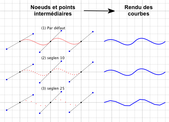
Figure 9: The segnb and seglen instructions used to optimize curve rendering. On the left are shown the nodes, control points, and intermediate points used to calculate the curves. On the right are the Bézier curves drawn by GEOD. Three examples are illustrated: (1) default settings, (2) with seglen 10, and (3) with seglen 25. In the third case, the Bézier curve is not rendered satisfactorily because there are too few intermediate points.

The seglen instruction has another effect: it modifies the behaviour of the bezier command itself. The bezier command cleans up Bézier curves whose nodes are too close together.

GEOD removes any node located at too short a distance from its neighbour. The minimum valid distance between two nodes, 5 metres by default, is controlled by the seglen instruction.

This filtering operation performed by GEOD removes artefacts. It is especially useful when animating Bézier curves.

The resolution command

There is another command, resolution, which controls the number of intermediate points used to construct a Bézier curve. Note that this command applies to all curves defined in a script.

  resolution distance

where distance is a value in metres specifying the minimum spacing between two intermediate points. By default, the resolution in GEOD is 1 metre. Increasing this value smooths the curves and removes small-scale details.

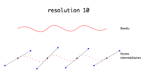
Figure 10: The resolution command. The instruction resolution 10 reduces the number of intermediate points used to draw the curve.

The tie subcommand

The tie subcommand makes it possible to construct a Bézier curve from other elements of the cross-section, such as points or other curves. This allows geometric constraints to be imposed on the drawing of the section.

Consider the example of a topographic profile on which outcrops of a layer boundary between the Cenomanian, in the footwall, and the Turonian, in the hanging wall, have been marked with the point command. To complete the section, these outcrops can be connected with a Bézier curve.

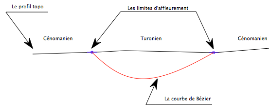
Figure 11: Construction of a Bézier curve from other elements of the cross-section. The Bézier curve, representing the layer boundary between the Cenomanian and the Turonian, is defined from two blue points, themselves attached to the topographic profile.

One possible procedure is:

  line
      x ... y ...
      x ... y ...
      name topo

point tie topo at x ... name ct0 point tie topo at x ... name ct1 bezier tie ct0 slope ... range ... tie ct1 slope ... range ...

The syntax is simple: tie is followed by the name of a point, previously defined with the name subcommand.

This technique has an important advantage.

If, later on, the topographic profile needs to be modified, it can be edited without worrying about the other elements of the cross-section. GEOD automatically updates the curve geometry while honouring the constraints defined with tie.

Another way to build the same section is to attach the new Bézier curve directly to the topographic profile, without first creating explicit point objects. Here again, the tie subcommand is used.

  bezier
      tie topo at x 100
          slope ...
          range ...
      tie topo at y 500
          slope ...
          range ...
      ...

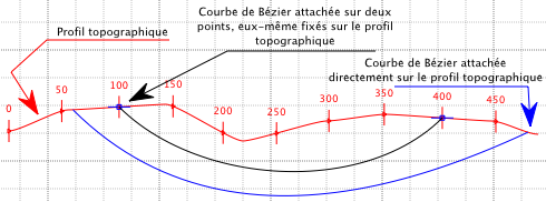
Figure 12: Bézier curves with nodes attached to points or to other curves.

There are five ways to attach a Bézier node to a line.

The fixed node is defined by its x coordinate.

  tie lineName at x value

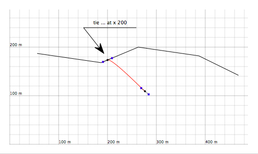
Figure 13: The instruction tie ... at x ...

The fixed node is defined by its y coordinate.

  tie lineName at y value

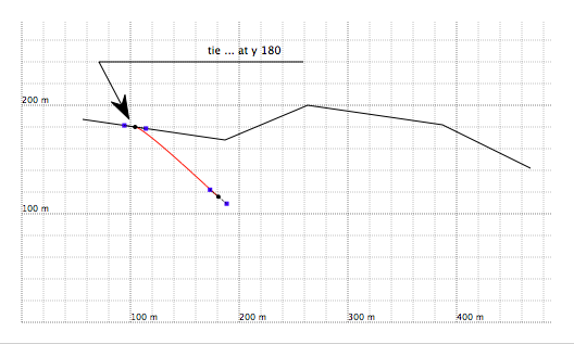
Figure 14: The instruction tie ... at y ...

The fixed node is defined by its curvilinear coordinate u.

  tie lineName at u value

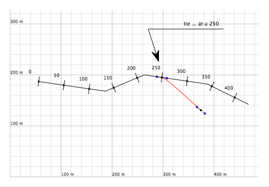
Figure 15: The instruction tie ... at u ...

The fixed node is defined by its depth.

Depth is measured from the intersection point between the line named lineName and the topographic profile. This option can be useful for constructing gallery or tunnel geometries.

  tie lineName at depth value

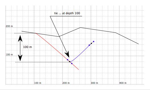
Figure 16: The instruction tie ... at depth ... The black curve is the topographic profile. The red line is a Bézier curve intersecting the topographic profile. The blue curve is a Bézier curve attached to the red curve at a depth of 100 metres, measured from the intersection of the red curve with the topographic profile.

The fixed node is attached to a node of another curve.

The node on the other curve, named lineName, is identified by an index number ranging from 1 to n, where n is the number of nodes on the curve.

  tie lineName at index value

The dir subcommand

The dir subcommand defines the position of a new node, not from explicit x and y coordinates, but relative to the position of the previous node.

  dir angle distance

where:

angle specifies the angular direction followed by the Bézier curve between the previous point and the new point. This angle is measured in degrees. A value of zero corresponds to a direction pointing to the right of the figure, that is, east. Note that, unlike the convention used for slope, leftslope, and rightslope, positive values, at least between 0° and 180°, direct the curve upward, that is, northward, while negative values, between -180° and 0°, direct it downward, that is, southward.
distance specifies the distance, in metres, between the previous point and the new point.

The fix subcommand

Like dir, the fix subcommand defines the position of a new node from the previous one. Its syntax is identical:

  fix angle distance

However, unlike dir, the angular direction is no longer measured relative to a horizontal line pointing to the right of the figure, but relative to the direction of the segment connecting the previous nodes of the Bézier curve.

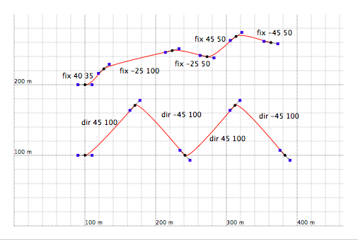
Figure 17: The dir and fix instructions used to construct Bézier curves.

The rel subcommand

The rel subcommand also defines a new node from its relative position with respect to the previous node, but this time in terms of horizontal and vertical displacements.

  rel deltax deltay

This places a node deltax metres to the right, if deltax is positive, or to the left, if deltax is negative, and deltay metres upward, if deltay is positive, or downward, if deltay is negative.

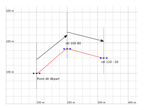
Figure 18: The rel subcommand used to insert nodes and position them by horizontal and vertical displacements.

Other instructions shared with the line command

Finally, the bezier command recognizes all instructions that can also be used with the line command, including:

graphic attributes, such as dashed and dotted for dashed and dotted rendering, color for line colour, width for line thickness, and backcolor for assigning a background colour to the line drawing, especially useful with dashed or dotted lines.
more advanced graphical attributes, such as line patterns, variable line styles as a function of curvilinear coordinates, and arrows.
other useful instructions, such as u0 to set the origin of the curvilinear coordinate scale, or nocrossing to remove loops.