GEOD

pattern (2)

Lithological patterns: the pattern command (2)

This section continues the presentation of the pattern instructions, with a particular focus on colour settings and the use of symbols.

Summary

Colour

The pattern command includes many instructions for specifying the colours of the different elements of a motif, including bars, markers, and background. It also allows transparency to be adjusted and different kinds of gradients to be created.

color

To replace the default black colour of the bars with another colour, use the color subcommand, which follows the usual syntax:

  color red green blue

where red, green, and blue are the RGB components of the colour. Their values must lie between 0 and 1. The triplet (0, 0, 0) defines black, and (1, 1, 1) defines white.

A predefined colour name may also be used:

  color colorName

where colorName must be replaced by a colour name recognized by GEOD. The list of available colours is given here.

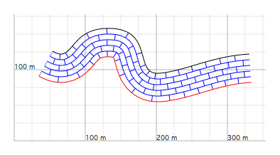
Figure 1: Blue pattern produced by the instruction color blue.

fillcolor

To assign a background colour to the pattern, use the fillcolor subcommand. Its syntax is strictly identical to that of color.

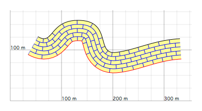
Figure 2: Pattern with a yellow background produced by the instruction fillcolor yellow.

alpha

The alpha instruction makes the pattern semi-transparent, or even completely transparent. This subcommand takes a single argument:

  alpha f

where f controls the transparency of the pattern and must take a value between 0 and 1. A value of 0 means full transparency, so the pattern is no longer visible, while a value of 1 means full opacity, so objects behind the pattern are completely hidden.

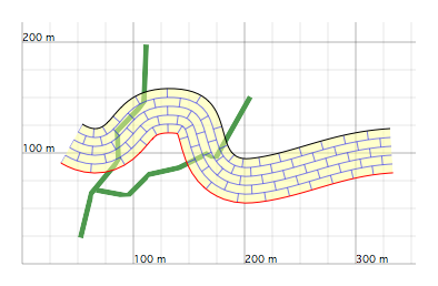
Figure 3: The same motif as in Figure 2, but with the instruction alpha 0.5. Two dykes have also been drawn in the background and appear more faded where they pass through the limestone series. This drawing device can be used to suggest that the intrusion took place not exactly in the section plane, but a few tens of metres behind it.

Note that changing the alpha parameter affects not only the coloured background of the pattern, but also all the bars and symbols it contains.

nalpha

The nalpha instruction makes it possible to draw a coloured background with a gradient. The gradient is calculated perpendicular to the layer boundaries, that is, along the direction of the normal vector n to the layer boundaries, hence the name nalpha.

This instruction must be followed by a list of values enclosed in parentheses, using a syntax that has already been encountered elsewhere.

To define the gradient, GEOD uses the transparency properties of the pattern and modulates them according to the relative position within the layer. For this purpose, GEOD uses the so-called normal coordinate, also denoted n.

n = 0 at the mother curve,
n = 1 at the daughter curve,
and between these two limits, n varies linearly.

For example, to create the motif shown in Figure 4, the following instruction was used:

  nalpha ( 0.5 at 0.2, 1 at 0.8 )

This may be interpreted as follows:

for n between 0 and 0.2, that is, near the mother curve, the alpha parameter is 0.5, so the yellow background appears very pale because it is mixed equally with the white background of the figure,
for n between 0.8 and 1, that is, near the daughter curve, alpha is 1, so the motif is fully opaque and the yellow colour is strongly saturated,
in the intermediate interval, from n = 0.2 to n = 0.8, alpha varies linearly from 0.5 to 1, that is, from semi-transparency to full opacity.

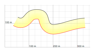
Figure 4: Gradient motif produced by the instruction above.

xalpha, yalpha, ualpha

The pattern command includes three additional instructions that can be used to create gradients:

xalpha computes the gradient as a function of the horizontal coordinate x,
yalpha computes the gradient as a function of the vertical coordinate y,
ualpha computes the gradient as a function of the curvilinear coordinate u of the mother curve.

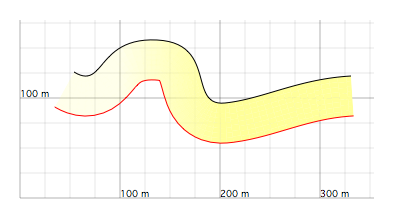
Figure 5: Pattern with a gradient produced by xalpha (0.2 at 100, 1 at 200).

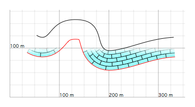
Figure 6: Pattern with a gradient computed as a function of the vertical coordinate y, using yalpha (1 at 50, 1 at 85, 0 at 100).

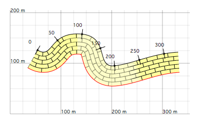
Figure 7: Pattern with a gradient computed as a function of the curvilinear coordinate u of the mother curve, using ualpha (1 at 100, 0.5 at 100, 0.5 at 250, 1 at 250).

The ualpha instruction can also be used to draw layers showing lateral facies variations, as in the example below.

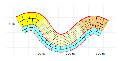
Figure 8: Layer with lateral facies variations. The mother curve is drawn as a thick red line. The other layer boundaries are obtained by offsets using the offset command. For the layer with lateral facies variation, the mother curve was offset in three pieces, a left segment, a central segment, and a right segment, using umin and umax. Each segment was decorated with its own pattern command. The transitions between the left and central parts and between the central and right parts are ensured by a ualpha instruction.

ralpha and calpha

The ralpha and calpha instructions are two subcommands used to create a radial gradient.

ralpha specifies the variation of the alpha parameter as a function of the radial coordinate r. This instruction follows the same general syntax as xalpha, yalpha, ualpha, and nalpha.

calpha specifies the position of the central point from which the radial coordinate r is calculated:

  calpha xc yc

where xc and yc are the x and y coordinates of this point.

For example, to compute the motif shown below, the following instructions were used:

  alternate
  levels 5
  fillcolor yellow
  ralpha (1 at 40, 0.0 at 100)
  calpha 134.0 133.0

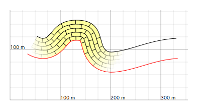
Figure 9: Pattern with a radial gradient centered on the hinge of the anticline.

Symbols

The pattern command can insert symbols between the bars and provides several instructions for controlling their appearance.

Marker types

To display a motif with symbols, simply use one of the following subcommands:

circle — circle
verti — vertical line
horiz — horizontal line
square — square
diamond — diamond
cross — cross
xcross — X-shaped cross
triangle — upward-pointing triangle
dtriangle — downward-pointing triangle
asterisk — asterisk
vee — V-shape
basevee — V resting on a horizontal line
dvee — inverted V
ltilda — tilde-like symbol
rtilda — reversed tilde-like symbol
crescent — upward-facing crescent
dcrescent — downward-facing crescent
char — character
icon — icon

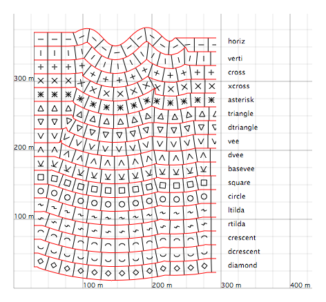
Figure 10: The different basic markers that can be used in patterns.

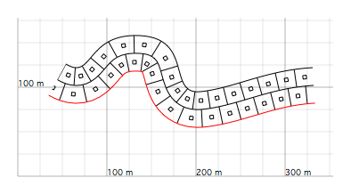
Figure 11: Pattern with square markers, produced by levels 2 alternate square.

Several remarks should be made about the use of these symbols:

by default, symbols are drawn as open markers. Their interior is transparent, and the outline is drawn with a one-pixel line.
markers are oriented according to the dip of the layers.
markers are always inserted between the lateral bars and the internal bars of the motif. Their arrangement is therefore controlled by all the instructions related to pattern bars, especially levels, vspacing, graded, sequence, spacing, alternate, oblique, double, period, spacing2, and base.
although these bars are necessary for arranging the markers, they can be hidden by using novertical to suppress the lateral bars and nohorizontal to suppress the internal bars.

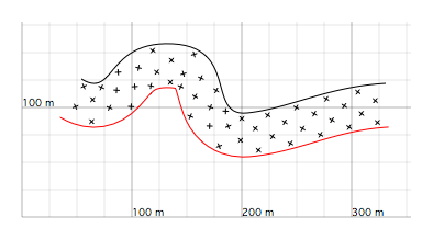
Figure 12: Pattern with X-shaped cross markers, produced by levels 4 alternate xcross novertical nohorizontal spacing 14. The lateral and internal bars used to position the symbols are hidden using novertical and nohorizontal.

it is not possible to use several different marker types directly in the same motif. For example, if the script contains square followed by circle, only circles will be displayed. The last marker instruction always overrides the previous ones.
some symbols have a polarity, that is, they have a distinct upper and lower part. This is the case for markers generated by triangle, dtriangle, vee, basevee, dvee, crescent, and dcrescent. The indications “upward” and “downward” given in the list above apply to a motif placed in a layer of normal polarity.

filled

The filled subcommand draws solid symbols instead of open ones. This naturally applies to closed or semi-closed markers such as circle, square, diamond, triangle, dtriangle, vee, basevee, dvee, crescent, and dcrescent.

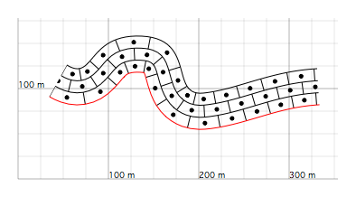
Figure 13: Pattern generated by levels 3 alternate circle filled. The filled instruction replaces the small circles by solid disks.

markercolor

The markercolor instruction specifies the colour of the symbol. It changes both the outline and the interior colour of the marker.

Its syntax follows the same conventions as other colour-setting instructions.

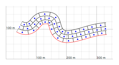
Figure 14: Pattern made of small solid blue triangles pointing upward.

backcolor

The backcolor subcommand allows the filling colour of the marker to be chosen independently from the colour of its outline. Its syntax is the same as for other colour-specification subcommands.

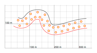
Figure 15: Pattern made of small yellow disks with a red outline. This was produced by markercolor red backcolor yellow filled.

markerwidth

The markerwidth instruction sets the thickness of the line used to draw the outline of the marker.

  markerwidth e

where e is the line thickness in pixels.

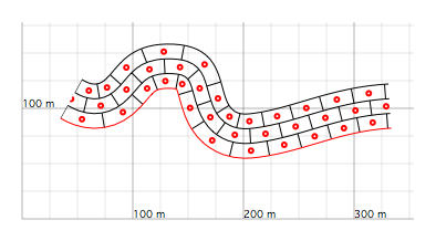
Figure 16: Pattern produced by levels 3 alternate markercolor red circle markerwidth 2.

markerperiod

The markerperiod instruction controls how frequently the symbols appear.

The lateral bars and the internal bars divide the motif into small cells, and by default each of these cells contains a symbol.

With markerperiod, one can specify that a marker should be placed only in one cell out of every two, or three, or another interval.

Its syntax is:

  markerperiod n

where n is the number of cells per marker.

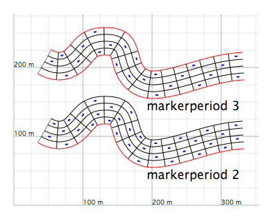
Figure 17: Illustration of markerperiod. Both patterns were produced with levels 4 spacing 20 markercolor blue markerwidth 2 horiz plus a markerperiod instruction. In the lower drawing, the symbol is present in one cell out of two, markerperiod 2, whereas in the upper drawing it is present in one cell out of three, markerperiod 3.

Another syntax is also possible:

  markerperiod n phase

The second argument, here called phase, shifts the cells that are filled or left empty.

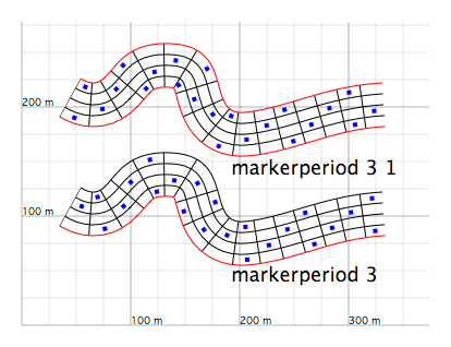
Figure 18: Shift of the filled cells. In both drawings, the motif is produced by levels 4 spacing 20 markercolor blue horiz markerwidth 4. The lower drawing uses markerperiod 3, whereas the upper drawing uses markerperiod 3 1.

size

By default, markers have a maximum size of 4 × 4 metres. The size instruction changes their dimensions. Its syntax is:

  size s

where s is the new size of the symbol in metres.

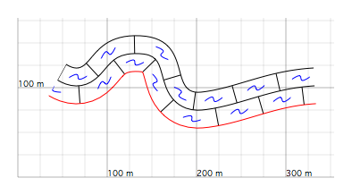
Figure 19: Illustration of the size subcommand. The motif is generated by levels 2 ltilda spacing 50 markercolor blue size 20 alternate.

If a large size is specified, any part of the marker extending outside the layer is automatically clipped by GEOD.

elastic and esize

The size instruction gives an absolute value for the size of the symbol. When the layer has variable thickness, especially when it is lens-shaped or tapers into a wedge, this instruction becomes inappropriate.

The pattern command provides two subcommands, elastic and esize, that deal with this situation.

The elastic instruction tells pattern to adapt the size of the marker to the size of the cell. By default, the dimension of the marker then becomes half the primary spacing defined by the spacing subcommand.

The esize instruction specifies the relative size of the marker:

  esize f

where f is a number expressing the relative size of the marker with respect to the primary spacing. For example, if f = 0.5, the symbol has a size equal to half of the primary spacing.

Normally, f takes a value between 0 and 1, but larger or even negative values may be used. In the latter case, the symbol is inverted.

In practice, elastic and esize make it possible to define truly elastic motifs that adapt automatically to the thickness of the layer.

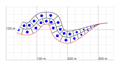
Figure 20: Variable-thickness layer, tapering into a wedge, with an elastic motif produced by levels 2 diamond spacing 25 markercolor blue filled alternate elastic esize 0.5.

char

Printed characters may also be used as motif markers. For this, use the char subcommand, followed simply by the character that will serve as the symbol. For example, to produce a motif based on the capital letter U, one may write:

  char U

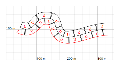
Figure 21: Alternating motif with markers in the form of the character “U”. The motif was generated by levels 2 spacing 35 markercolor red size 12 alternate period 2 spacing2 1.5 char U.

icon

Small icons may also be used as markers. For this, use the icon subcommand followed by the name of the file containing the image.

For example, to produce the motif shown below, the following instruction is used:

  icon "a.tif"

where a.tif is the file name.

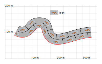
Figure 22: Motif produced by levels 2 spacing 40 fillcolor ltgray icon "a.tif".

markerscale

The markerscale instruction deforms a marker by a pure scaling transformation. It can be used in two different forms. The first is:

  markerscale s

where s is the enlargement factor, if s > 1, or the reduction factor, if s < 1. In this case, markerscale is simply a dilation or contraction.

The second, more flexible form is:

  markerscale sx sy

where sx and sy are the horizontal and vertical scaling factors respectively. This transformation is applied before the marker is rotated according to the dip. In this way, markerscale makes it possible to generate new marker shapes from the basic symbols listed above. For example, it can be used to produce:

ellipses from circles, for example circle markerscale 1.4 0.7,
rectangles from squares,
more strongly or more weakly curved tilde-like symbols or crescents.

The markerscale subcommand can also be applied to character markers created with char or icon markers created with icon.

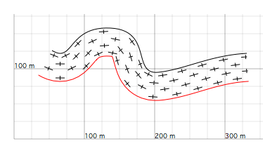
Figure 23: Pattern with stretched cross-shaped symbols produced by markerscale 1.3 0.6. The other instructions used are levels 4 spacing 30 size 10 cross alternate novertical nohorizontal.

random

The random instruction produces motifs with a more irregular appearance. It exists in three forms, random position, random orientation, and random size, which may be used separately or together.

  random position

places the markers randomly within their cells. Each marker nevertheless remains confined to its own cell, whose dimensions are controlled by the instructions presented in the section on pattern bars.

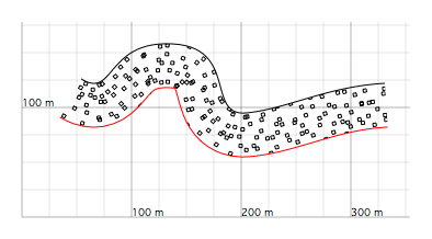
Figure 24: Motif generated by random position. The following instructions were used: levels 5 spacing 20 square random position novertical nohorizontal size 3.

  random orientation

rotates each marker randomly about its centre.

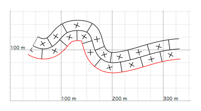
Figure 25: Motif generated by random orientation. The motif was produced by levels 2 spacing 40 cross random orientation size 12 alternate.

  random size

produces a motif with symbols of random size.

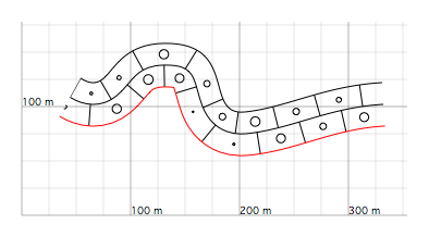
Figure 26: Motif generated by random size. The motif is produced by levels 2 spacing 40 circle random size size 6 alternate.

The intensity of the random fluctuations produced by these instructions may also be adjusted:

  random position f
  random orientation f
  random size f

where f is a positive number between 0 and 1:

for f = 1, the corresponding property, position, orientation, or size, fluctuates in a fully random way,
for f = 0, the fluctuations are suppressed and the effect of random disappears,
for intermediate values of f, the fluctuations progressively decrease as f approaches 0.

By combining different random instructions, a great variety of random motifs can be produced. To densify the pattern, one typically uses a large number of levels and a small spacing.

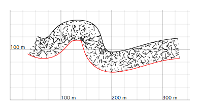
Figure 27: Motif produced by levels 7 spacing 5 horiz random position random orientation random size novertical nohorizontal size 6 alternate.

sand

The sand subcommand produces a random motif made of small circles. Unlike the other markers, this motif does not depend on the bar-setting instructions.

In its simplest form, this instruction is used without any argument and produces the motif illustrated below.

  sand

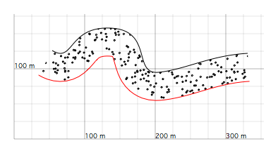
Figure 28: Motif produced by sand novertical nohorizontal.

On average, this subcommand places 30 markers in an area 100 metres wide, and each circle has a size of 2 pixels.

Three other syntactic forms are also possible:

  sand density

  sand density grainSize

  sand density grainSize heterometry

where density, grainSize, and heterometry are parameters affecting respectively the density, size, and grain-size distribution of the motif.

The parameter density sets the number of grains in a zone 10 metres wide, the default value being 3. The parameter grainSize specifies the grain diameter, 2 pixels by default. The parameter heterometry introduces random variations in grain size. By default, heterometry = 0, so all grains have the same size. The larger this parameter, the wider the size range of the grains.

Different examples of the sand instruction are shown below.

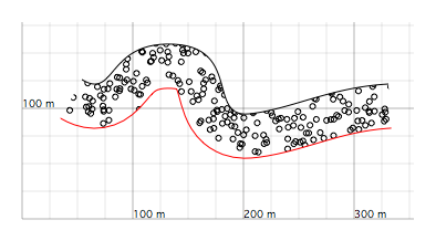
Figure 29: Motif produced by novertical nohorizontal sand 3 5.

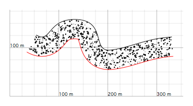
Figure 30: Motif produced by novertical nohorizontal sand 10 2 0.3.