GEOD
shift
Translating a curve with the shift command
The shift command defines the translated copy of a curve and provides an alternative to the offset command for constructing a geological layer. It is especially useful for drawing similar folds.
Summary
- The shift command
- Defining the translation vector with Cartesian components
- Defining the translation vector with polar components
- Drawing similar folds
- Translation vectors varying with curvilinear coordinates
- Options and special cases
- Discontinuities
- Optimizing the rendering of translated curves
- Removing self-intersections with nocrossing
- Eliminating intersections between homologous segments with method
The shift command
The shift command constructs the translated copy of a given curve, called the parent curve. The parent curve may be any type of curve, including a polyline, a Bézier curve, an offset curve, or any other curve available in GEOD. As with the offset command, the combination of the parent curve and its translated copy can then be used to define a new geological layer.
The translation vector may be defined:
- either by its horizontal and vertical components,
- or by its polar components, that is, direction and distance.
Defining the translation vector with Cartesian components
The syntax is:
shift lineName dx dy
where:
- lineName designates the parent curve. It is the name previously assigned to the curve with the name instruction.
- dx and dy are respectively the horizontal and vertical components of the translation vector.
The parameter lineName is optional. If it is omitted, GEOD implicitly translates the last curve defined before the shift instruction.
Important note: a positive value of dx shifts the new curve to the right, while a positive value of dy shifts it downward. In this respect, the same convention is used as for the offset command.
Example:
shift 20 30
This shifts the last curve defined before the shift instruction by 20 metres to the right and 30 metres downward.
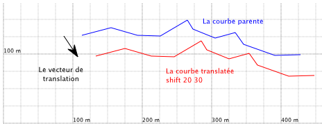
Figure 1: Curve translation with the shift command. The parent curve is shown in blue and the translated curve in red. The translation vector defined by shift 20 30 corresponds to 20 metres to the right and 30 metres downward.
Defining the translation vector with polar components
The translation vector may also be defined in terms of direction and distance, that is, in polar form.
The syntax is then:
  shift lineName angle distance
      polar
where:
- lineName designates the parent curve. This argument is again optional.
- angle is the angular direction of the translation vector. The angle is measured in degrees, with zero pointing east, and increasing clockwise. Thus, a value between 0° and 180° shifts the curve downward.
- distance is the length of the translation vector in metres. A negative value may also be used, in which case the translation takes place in the direction opposite to that indicated by angle.
- polar is a subcommand that must appear somewhere in the definition of the translated curve. It tells GEOD to interpret angle and distance as polar components, rather than as Cartesian components.
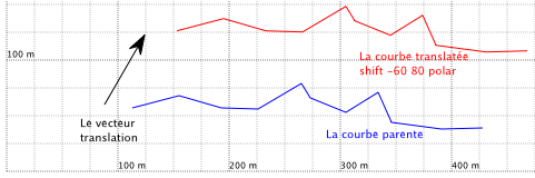
Figure 2: Defining the translation vector with polar components.
Drawing similar folds
The shift command is particularly well suited to drawing similar folds. In this case, the translation vector is usually defined in polar form.
The example below is built from a Bézier curve.
The Bézier curve is defined from a few nodes placed midway along the fold limbs. Each of these nodes is characterized by the same dip, 60°, and by a large range of 200 metres.
The other layer boundaries, above and below the Bézier curve, are obtained by successive translations using the shift command.
It should be noted that the translation vector must be oriented slightly differently from the dip direction of the nodes. Otherwise, half of the fold limbs would become excessively compressed.
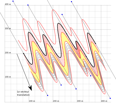
Figure 3: Drawing similar folds with shift commands. The black curve is a Bézier curve. All the other layer boundaries are translated curves. The nodes of the Bézier curve are also shown with their ranges. The black arrow indicates the translation vector. Its direction, 68°, is slightly different from the node direction, 60°.
Translation vectors varying with curvilinear coordinates
It is possible to define a translation vector whose components depend on the position of the point being translated on the parent curve. For this, curvilinear coordinates are used.
If the translation vector is defined by its Cartesian components, dx and dy, these components may vary as a function of u. For example:
  shift
      (0 at 0, 100 at 300)
      50
In this example, the horizontal component of the translation vector is defined by the variable function shown in parentheses, while the vertical component remains constant at 50. The horizontal variation is linear, and the values given between parentheses constrain this component at specific points. GEOD then calculates the horizontal component by interpolation between these values.
The resulting translated curve is shown in the figure below.
The vertical component may also depend on u, and both components may vary simultaneously.
Spatial variables defined with the set ... to var command may also be used, as in the following example:
  set vy to var
      (-50 at 0, 0 at 300)
Here, a spatial variable named vy is defined.
To use this spatial variable in a shift instruction, the keyword with is used:
  shift 20
      with vy
In this example, the horizontal component is fixed at 20, while the vertical component is given by the variable vy.
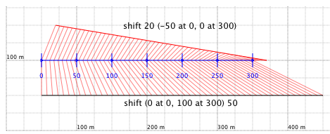
Figure 4: Translating curves with non-constant translation vectors. The parent curve is shown in blue, and its curvilinear coordinate scale is displayed with the graduate instruction. Two translations have been applied to it, producing two curves, one black and one red, according to the shift instructions shown. The points used for the translation and the resulting points are connected by segments displayed with pattern debug.
Non-constant translation vectors may also be defined in polar form. An example is shown below.
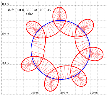
Figure 5: Curve translation by a vector of constant length, 45 metres, but variable angular direction. The blue curve is the parent curve, and the translated curve is shown in red. This figure could be used to illustrate the cycloidal path of a satellite around a planet.
Another advantage of variable translation vectors is that they can be used to construct similar folds with schistosity fans. The angular component of the translation vector can be varied alternately between the left and right limbs of folds to produce these characteristic deformation patterns.
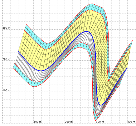
Figure 6: Similar fold constructed by translations with a translation vector of variable angular direction. The parent curve, in blue, is a Bézier curve and has been translated several times to produce different variants of folded layers with schistosity refraction.
Options and special cases
This section deals only with specific problems and special cases that may arise with the shift command.
Discontinuities
The shift command can handle discontinuities present in the parent curve. These discontinuities are created with the gap instruction. See polygonal lines and Bézier curves.
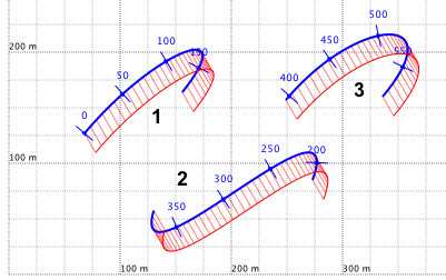
Figure 7: Translating a curve with discontinuities. The parent curve is shown in blue, the translated curve in red, together with the segments linking homologous points between the parent curve and the translated curve. The parent curve is divided into three separate parts. Curvilinear coordinates are displayed with the graduate instruction.
Optimizing the rendering of translated curves
A translated curve is made of a series of small segments. To speed up the rendering of a cross-section, it may be useful to adjust their number. The shift command duplicates each intermediate point of the parent curve. It is therefore on the parent curve itself, when it is a polyline or a Bézier curve, that the number of intermediate points can be reduced using the segnb and seglen instructions. See the section on polygonal lines and the section on Bézier curves.
An example is shown below.
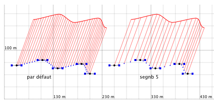
Figure 8: Optimized rendering of translated curves. The blue dashed line is the Bézier curve used as the parent curve. The translated curve is shown in red, together with the segments linking intermediate points of the parent curve and the translated curve. The nodes and control points of the Bézier curve are also shown. On the left is the default rendering. On the right, the rendering has been optimized with segnb 5, which reduces the number of intermediate points used to draw both the Bézier curve and the translated curve.
Removing self-intersections with nocrossing
Translation with a non-constant translation vector may generate situations in which the translated curve has undesirable self-intersections, just as can happen with offset curves produced by the offset command. GEOD provides subcommands to deal with these problems.
A first step is to use the nocrossing subcommand, which activates the automatic removal of loops. This instruction is available for all types of lines in GEOD.
nocrossing
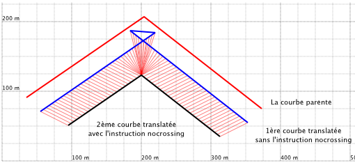
Figure 9: Illustration of the nocrossing subcommand applied to translated curves. The parent curve is shown in red and is used to construct two translated curves with non-constant translations. The first translated curve, in blue, shows an unwanted line crossing in the fold hinge. The second translated curve, in black, is drawn correctly thanks to the nocrossing subcommand.
Eliminating intersections between homologous segments with method
In some cases, nocrossing is not sufficient, and it becomes necessary to detect and eliminate intersections between the segments linking homologous points on the parent curve and on the translated curve. For this, the method subcommand is used. It was already introduced in the section on offset curves produced by the offset command.
The method subcommand is written as:
method value
where value may be either 1 or 2, and selects the algorithm to apply. More detailed explanations are given in that section.
An example is shown in the figure below. In this example, nocrossing has no effect because the translated curve does not intersect itself. The problem comes from the crossing of homologous segments, and it is the instruction method 2 that solves the rendering issue.
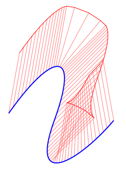
Figure 10: Drawing a folded layer. The Bézier curve shown in blue is the parent curve, and the translated curve is shown in red, together with the segments linking homologous points on the parent and translated curves. The translation is 120 metres upward, but with an orientation varying as a function of the curvilinear coordinate u of the translated point on the parent curve. The rendering is poor in the syncline hinge, as shown by the intersections of the segments.
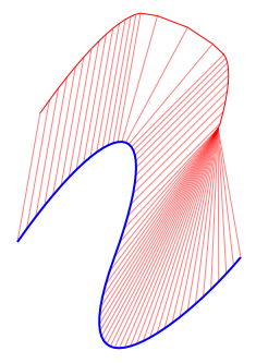
Figure 11: The same figure as above, but with the instruction method 2 applied to remove the segment intersections.
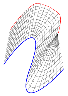
Figure 12: Final rendering of the folded layer after applying a lithological pattern.