FIT-OIL
Microthermometric analysis of hydrocarbon inclusions
Table of contents
- Introduction
- Notations
- About FIT-Oil
- In which order should the different FIT-Oil modules be used?
- A few words about FIT-Oil
- The tutorial
- 1. How to calculate an alpha-beta curve
- 2. How to select an alpha-beta fluid
- 3. How to use alpha-beta correlations
- 4. How to calculate immiscibility loops
- 5. Isochors
- 6. How to determine trapping conditions
- 7. Volume-temperature diagrams
- 8. To enter inclusion data
- 9. To plot volumetric data
- 10. To define fluid models
- 11. To use a fluid model
- 12. To generate a fluid model from an alpha-beta model
Introduction
FIT-Oil is a software package designed for the study of petroleum fluid inclusions.
It uses:
- microthermometric data (homogenisation temperature),
- measurements of bubble filling degree, which can be determined accurately by confocal scanning laser microscopy at various temperatures.
FIT-Oil allows users:
- to calculate liquid-gas phase transitions and draw phase diagrams for hydrocarbon mixtures,
- to obtain information about the nature and composition of the petroleum trapped in fluid inclusions (petroleum type, GOR, API°),
- to reconstruct the paleo-temperature and pressure conditions of petroleum migration in oil fields,
- to infer information about petroleum evolution and past processes that occurred in the reservoir (pressure or temperature variations, gas inputs, gas or water leaching, etc.), or in the inclusions after petroleum trapping (leakage, deformation).
FIT-Oil is therefore a useful tool for specialists working on fluid inclusions.
FIT-Oil is provided without warranty and must be used at the user’s own risk.
Notations
- T: temperature,
- P: pressure,
- Th: homogenisation temperature,
- V: bubble filling degree in the fluid inclusion, expressed as a volume percentage,
- Fv: bubble filling degree,
- alpha: one compositional parameter of petroleum,
- beta: another compositional parameter of petroleum.
About FIT-Oil
FIT-Oil is a modular application composed of five main modules, which can be used independently or in combination.
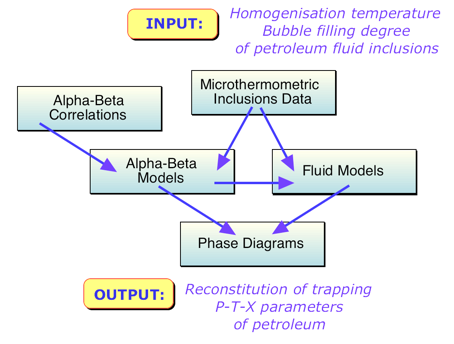
The main modules of FIT-Oil
1. Alpha-beta models
FIT-Oil uses a specialised compositional model, referred to as the alpha-beta model (Montel, 1993), to describe the physico-chemical properties of petroleum, including its immiscibility loop in a pressure-temperature diagram, its GOR, and its API degree.
The alpha-beta model offers two main advantages:
- it uses only two compositional parameters, alpha and beta, to describe petroleum composition,
- it can represent the properties of most common petroleum types.
When applied to petroleum fluid inclusions, FIT-Oil attempts to determine the alpha and beta parameters that best fit the measured microthermometric data (homogenisation temperature and gas bubble filling degree). However, there is no unique solution.
For each inclusion studied, FIT-Oil calculates a curve known as the alpha-beta curve, which represents the set of possible solutions. FIT-Oil displays this curve in an alpha-beta plot.
The range of possible solutions can be further constrained by incorporating additional information, such as API° values obtained from microspectrofluorimetry.
2. Phase diagrams
This module calculates the pressure-temperature phase diagrams of petroleum fluids.
These phase diagrams include:
- isopleths,
- isochores in both biphasic and monophasic fields,
- trapping points.
This module also allows the calculation of bubble filling degree as a function of temperature.
Phase diagrams can be produced:
- either from an alpha-beta model,
- or from user-defined theoretical fluids, referred to in the documentation as fluid models.
3. Input of microthermometric inclusion data
This module is used to enter microthermometric data for inclusions.
It includes:
- homogenisation temperatures,
- bubble filling degrees measured at several temperatures.
4. Alpha-beta correlations
Alpha-beta correlations are collections of alpha-beta values determined for characteristic petroleum types.
These correlations help users select realistic alpha and beta values for oils trapped in fluid inclusions.
5. Fluid models
The last module uses fluid models.
Fluid models are mixtures, generally made up of 10 to 20 hydrocarbon pseudo-components, whose thermodynamic parameters can be adjusted.
They provide additional flexibility for the compositional modelling of petroleum fluids, in a way similar to PVTSim.
In other words, this is an alternative to alpha-beta models.
Fluid models may also be used when compositional analyses of the trapped petroleum are available.
It is also possible:
- to generate a fluid model from an alpha-beta model,
- to modify it according to your needs,
- to generate a fluid model by flash calculation from another model, either an alpha-beta model or another fluid model.
Once a fluid model has been defined, FIT-Oil can calculate phase diagrams and volumetric plots for it.
In which order should the different FIT-Oil modules be used?
There are several ways to use FIT-Oil. If you have only a small number of inclusions, the most common workflow is as follows:
- first switch to the alpha-beta plots module,
- enter the microthermometric data (Th, Fv, and gas composition if available),
- calculate the alpha-beta curves and select realistic alpha-beta parameters,
- using the selected alpha-beta values, draw the P-T phase diagrams including isopleths and isochores; test several sets of alpha-beta parameters,
- then determine trapping pressures from the homogenisation temperatures of coeval aqueous fluid inclusions.
Use the microthermometric input module if you have a large number of inclusions. This module allows you to assign names and abbreviations to inclusions.
Use the alpha-beta correlations module if you wish to include your own alpha-beta correlations.
Use the fluid model module if alpha-beta models do not suit your needs. You can then calculate phase diagrams for these theoretical fluids.
Finally, all data, values, tables, and diagrams calculated by FIT-Oil can be exported to Microsoft Excel, where they can be further processed and printed.
A few words about FIT-Oil
FIT-Oil is a multi-platform application. It can run on Windows and Mac OS X systems. There is also a non-GUI version, which can be compiled for any computer system.
FIT-Oil is the first in a planned series of software packages for fluid inclusions, grouped under the name FIT (Fluid Inclusions Thermodynamics), which will also include:
- FIT-Gas, for the study of the gaseous phase of fluid inclusions (CO2-CH4-N2),
- FIT-Aq, for the study of aqueous inclusions (H2O-CO2-CH4-NaCl).
FIT-Oil also uses the LOTHER calculation library (Library Oriented Object for THERmodynamic calculations) to compute liquid-gas phase equilibria and thermodynamic fluid properties using equations of state (Thiéry, 1996).
References
- A new object-oriented library for calculating high-order multivariable derivatives and thermodynamic properties of fluids with equations of state. R. Thiéry. Computers & Geosciences, 22 (1996), 801-815.
- The IAPWS formulation 1995 for the thermodynamic properties of ordinary water substance for general and scientific use. W. Wagner and A. Pruss. J. Phys. Chem. Ref. Data, 31 (2002), 387-535.
The FIT-Oil package
The FIT-Oil package contains several components:
- the FIT-Oil software,
- the documentation,
- demonstration files,
- a tutorial.
FIT-Oil is available for Windows and Mac OS X.
The tutorial
A tutorial has been developed using OxGo software for creating multimedia-rich documents, including pictures, text, and animations.
It presents:
- an introduction to petroleum inclusions, their nature, and their formation,
- the various analytical methods (spectrometry, microthermometry, volumetry, gas chromatography),
- the alpha-beta compositional model used as a proxy for complex natural petroleums,
- the FIT-Oil method for reconstructing paleo-pressure and paleo-temperature trapping conditions and estimating petroleum composition.
[A short preview of the tutorial in PDF format is available here (French version).]
[A visual overview of the FIT-Oil interface is also available here.]
Here are the main topics covered by FIT-Oil.
1. How to calculate an alpha-beta curve
Alpha-beta curves are estimated from the Th and Fv parameters.
Definitions:
- Th: homogenisation temperature of the oil-bearing fluid inclusion,
- Fv: bubble filling degree at ambient temperature.
FIT-Oil uses a simple compositional model, referred to as the alpha-beta model (Montel, 1993), to describe the physico-chemical properties of petroleum.
This model is based on two parameters:
- alpha, related to the content of high-molecular-weight compounds,
- beta, related to the content of volatile molecules such as methane and C2-C6 compounds.
Homogenisation temperature and bubble size in petroleum fluid inclusions depend on composition, and therefore on the alpha-beta parameters.
However, it is not possible to determine both alpha and beta unambiguously from Th and Fv alone. FIT-Oil can only provide a range of probable values: these are the alpha-beta curves.
This range can be further constrained using other data, such as correlations, GOR, or API°.
To calculate an alpha-beta curve
- Select the Alpha-Beta Model > New Alpha-Beta Plot... menu item.
- In the Alpha-Beta Curves panel of the floating window, enter the microthermometric properties of the inclusion in the fields Homogenisation temperature, Bubble size, Temperature of volume measurement, CO2, N2, and H2S, and specify the type of homogenisation (liquid or gas).
- Click the Calculate the Beta-Alpha Curve button.
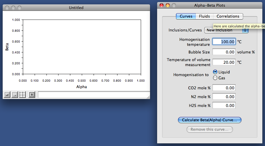
Alpha-beta plot window and controls
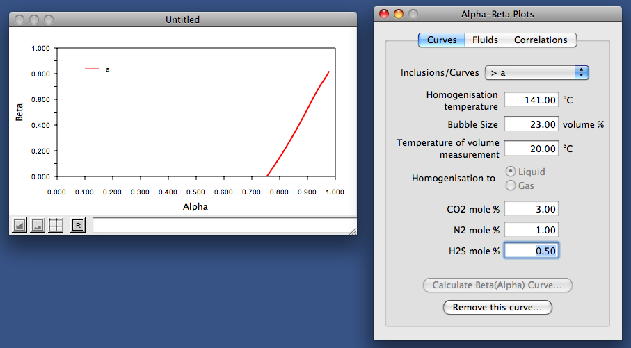
Calculation result and naming of the new alpha-beta curve
The calculation generally takes about 5 to 10 seconds. FIT-Oil displays a progress bar and then asks the user to name the newly calculated alpha-beta curve.
2. How to select an alpha-beta fluid
Alpha-beta fluids are points selected in alpha-beta plots. They can be stored for later use.
To select an alpha-beta fluid
- Select the Alpha-Beta Fluids panel of the Alpha-Beta Plots floating window.
- Enter the alpha and beta values in the corresponding fields.
- If you want the fluid to belong to a calculated alpha-beta curve, check The fluid is on a curve and specify the relevant curve.
- Click the New Fluid button.
- FIT-Oil displays a marker corresponding to the selected alpha-beta point.
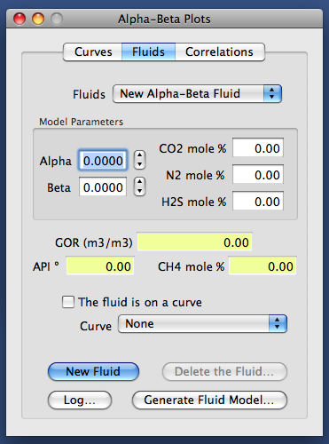
Selecting an alpha-beta fluid
GOR, API degree and CH4 content
GOR, API degree, and CH4 content are automatically calculated and displayed whenever alpha or beta changes. This helps users choose appropriate alpha and beta values.
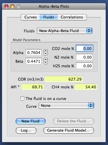
Automatic display of GOR, API degree and CH4 content
To generate a fluid model from selected alpha-beta markers
Click the Generate a fluid model button. This creates a fluid model document whose hydrocarbon composition can later be modified.
Note: it is often easier to select alpha and beta directly by clicking on the alpha-beta diagram. A right-click displays a contextual menu; select Set a marker to choose an alpha-beta point.
3. How to use alpha-beta correlations
Alpha-beta correlations provide a small database of alpha-beta parameters determined for natural petroleums. These values are calculated to reproduce the phase diagrams of these fluids as closely as possible.
They can therefore be used as a reference for selecting probable alpha-beta values for fluid inclusions.
To display an alpha-beta correlation
- Select the Correlations panel of the Alpha-Beta Plots floating window.
- Click the Display a new correlation button.
- Choose a correlation file. Correlation files use the suffix .abe.
- FIT-Oil displays the alpha-beta values in the alpha-beta plot.
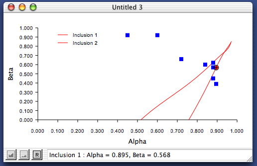
Example of an alpha-beta correlation
In the example above, the correlation was calculated from typical petroleum types: black oils, volatile oils, gas condensates, wet gas, and dry gas.
The contents of an alpha-beta correlation
It is possible to examine the contents of a correlation:
- Select Alpha-Beta Model > Edit Correlation...
- A table is displayed, in which each row corresponds to a petroleum type.
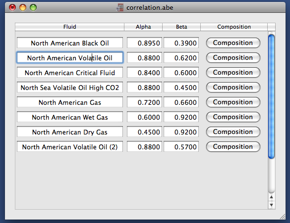
Table of alpha-beta correlation values
The composition of an alpha-beta fluid
To view the theoretical molecular composition of an alpha-beta fluid used internally by FIT-Oil, click the Composition... button.
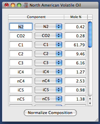
Theoretical composition window for an alpha-beta fluid
Iso-GOR and iso-API curves
API° and GOR are parameters commonly measured for reservoir petroleums. Their dependence on alpha and beta can be visualised on alpha-beta plots and used as a guide when selecting alpha-beta parameters.
To display iso-GOR curves, click the Show iso-GOR curves checkbox.
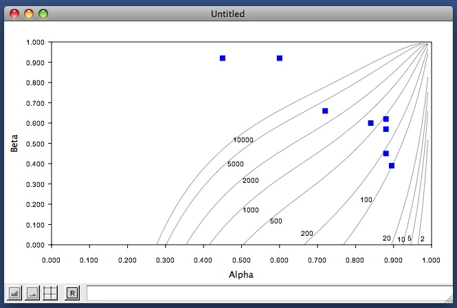
Iso-GOR curves in an alpha-beta plot
To display iso-API curves, click the Show iso-API curves checkbox.
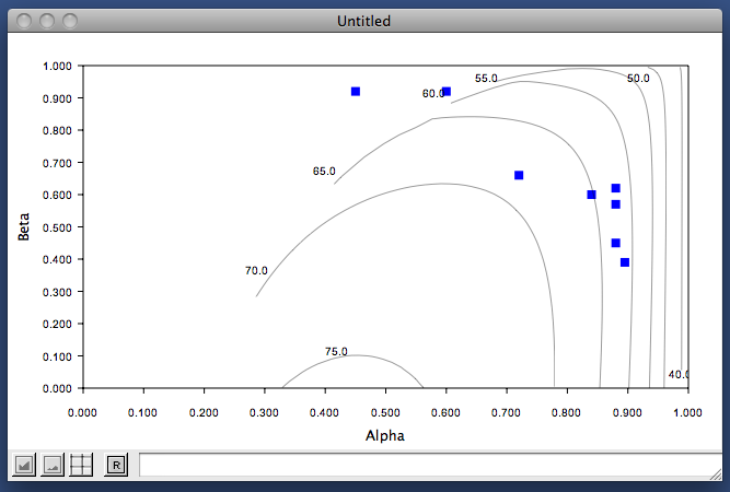
Iso-API curves in an alpha-beta plot
4. How to calculate immiscibility loops
After selecting alpha-beta parameters, the phase diagram can be calculated.
- Select Phase Diagrams > New P-T diagram...
- A new window opens with an empty P-T phase diagram and a floating window named Phase Diagrams.
This floating window contains four panels:
- Isopleths,
- Isochors,
- Trapping,
- Clean.
These panels group the main tasks involved in constructing the phase diagram.
To calculate an isopleth
- Click Use Alpha-Beta Model.
- Select an alpha-beta fluid in the list box, or enter alpha and beta directly.
- Optionally specify the mole % of CO2, N2, and H2S.
- Click Calculate the isopleth.
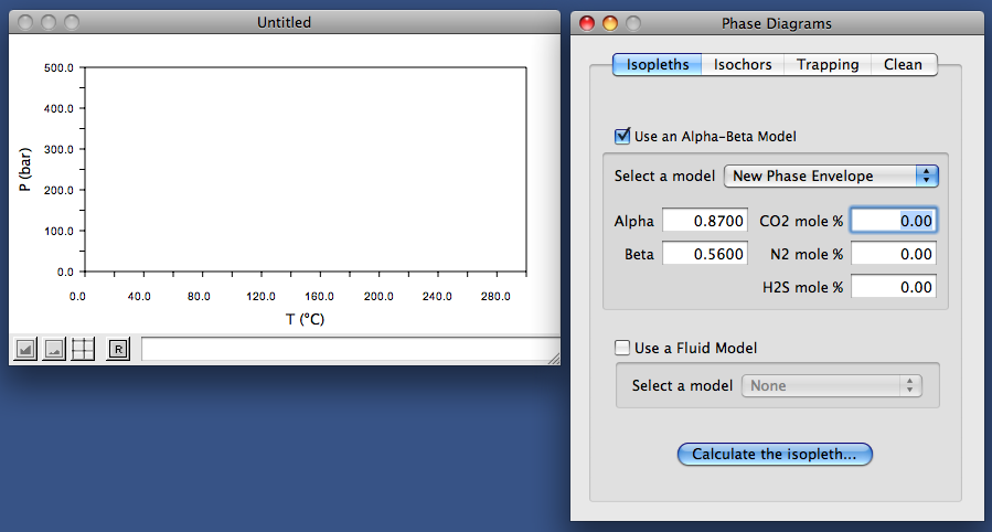
Isopleth calculation controls
The immiscibility loop
The liquid-gas immiscibility loop is calculated and displayed immediately in the P-T phase diagram.
The filled circle on the isopleth represents the liquid-gas critical point. The loop separates the biphasic liquid-gas field from the monophasic field.
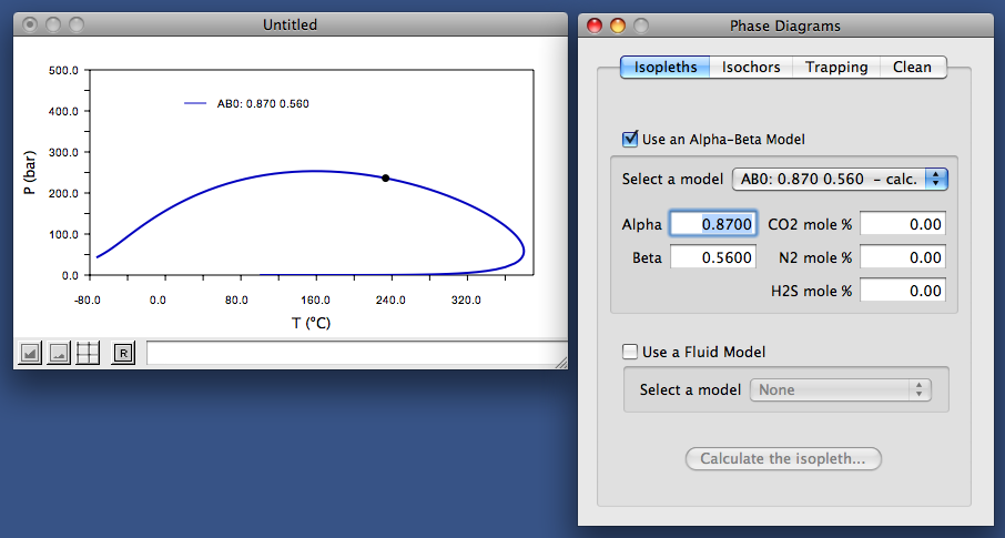
Liquid-gas immiscibility loop in a P-T diagram
To modify axis ranges
Select Edit > Axis ranges... to specify the new horizontal and vertical axis ranges.
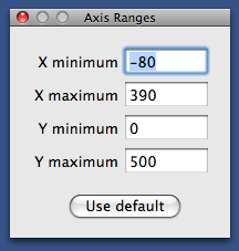
Axis range dialog box
It is also possible to click and drag a selection rectangle on the plot and then use the magnification button in the lower-left corner of the window.
5. Isochors
To calculate an isochor
- Switch to the Isochors panel of the Phase Diagrams window.
- Select one of the calculated isopleths in the Model list.
- Specify the microthermometric properties of the inclusion:
- its homogenisation temperature in °C,
- and its type of homogenisation (liquid or gas).
- Click the Calculate the isochor button.
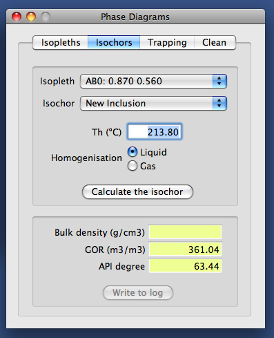
Isochor calculation panel
The isochor
FIT-Oil immediately draws the corresponding isochor in the phase diagram. This line represents the pressure-temperature path followed by the inclusion and intersects the immiscibility loop at the homogenisation point.
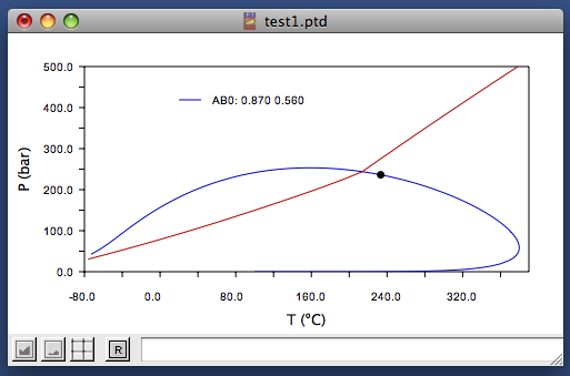
Isochor drawn in the phase diagram
The calculated isochor is also listed in the Isochors panel. It is assigned a new name combining the alpha-beta model abbreviation and the homogenisation temperature.
Isochor properties
The Isochors panel also shows additional information for the selected isochor:
- bulk density of the inclusion (g/cm3),
- bulk molar volume (cm3/mol),
- GOR (Gas-Oil Ratio).
To display these data:
- select the isochor in the inclusion list,
- browse through the list to compare isochor properties.
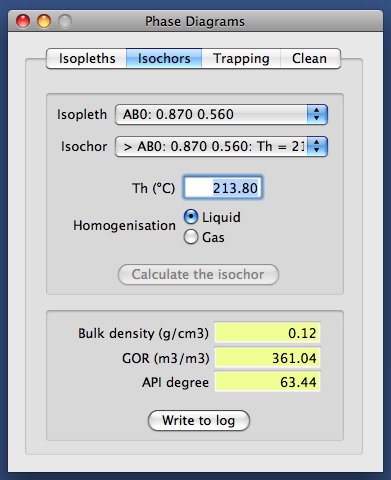
Isochor properties displayed in the interface
Thermodynamic properties
If necessary, detailed thermodynamic data can be written to an ASCII log file by clicking the Write to Log button.
In addition to other data, the log includes:
- saturation pressure (bar),
- GOR and API° calculated by the Standing & Katz method,
- molar mass (g/mol), density (g/cm3), and specific volume (cm3/g) of the sampled liquid under STP conditions (15°C and 1 bar).
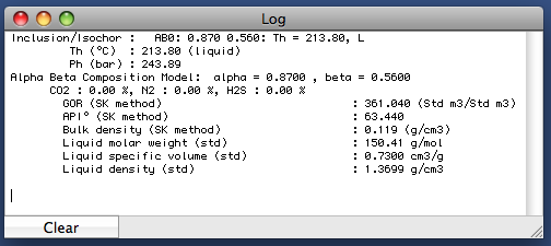
Detailed thermodynamic properties written to the log
6. How to determine trapping conditions
The calculated isochor provides an indication of the paleo-pressure and paleo-temperature conditions at which the petroleum was trapped in the fluid inclusion. The trapping point necessarily lies somewhere on this line in the monophasic field.
In some cases, coeval aqueous inclusions are also present. Their homogenisation temperature may indicate the trapping temperature of the petroleum inclusions, allowing the trapping pressure to be read directly.
To determine trapping pressure
- Switch to the Trapping panel of the Phase Diagrams floating window.
- Select the isochor in the list box, or click directly on it in the pressure-temperature plot.
- Enter the homogenisation temperature of the aqueous inclusion in °C.
FIT-Oil immediately draws a thin vertical pink line in the P-T diagram, and the trapping pressure in bar is displayed in the corresponding field.
This trapping line is temporary and moves automatically when the homogenisation temperature of the aqueous inclusion is modified.
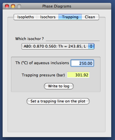
Temporary trapping line in the P-T diagram
To permanently fix the trapping line in the phase diagram
- Click the Set a trapping line button.
- The trapping line is then fixed permanently and stored in the document file.
To retrieve the results
- Click the Write to Log button.
- FIT-Oil writes all calculated results to the log file, including the inclusion name, trapping pressure, compositional model used, and homogenisation temperature of aqueous inclusions.
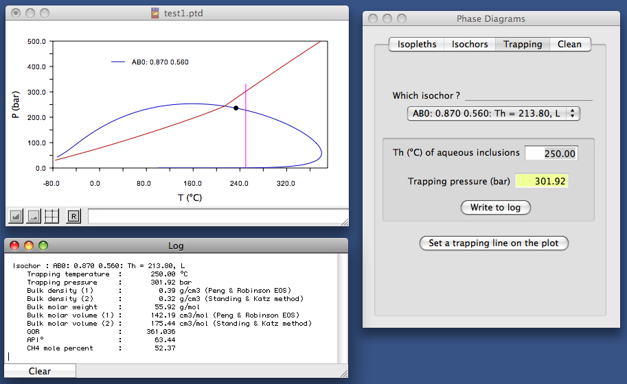
Trapping results written to the log
Bulk densities are calculated using two methods: the Peng-Robinson equation of state and the Standing-Katz method. Both methods have limitations.
The Peng-Robinson equation of state yields only moderate estimates of liquid density, whereas the Standing-Katz correlation is not reliable above 200°C.
7. Volume-temperature diagrams
FIT-Oil can also draw the evolution of bubble filling degree (in volume %) as a function of temperature.
This curve is calculated in the biphasic liquid-gas field and makes it possible to compare calculated values with measurements performed on inclusions, for example by confocal scanning laser microscopy.
- Select V-T plots > New V-T plot...
- FIT-Oil displays a new window showing an empty Bubble Filling Degree (% volume) versus Temperature (°C) diagram.
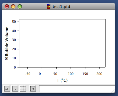
Empty V-T plot window
FIT-Oil also displays a floating window used to construct the V-T diagram by plotting calculated volumetric curves together with inclusion data.
To add a volumetric curve calculated by FIT-Oil
- Switch to the V-T curves panel of the V-T plot floating window.
- The left list contains available calculated isochores not yet inserted into the diagram.
- The right list contains the isochores already plotted.
- Select the isochor to plot in the left list.
- Click Plot Isochor >>.
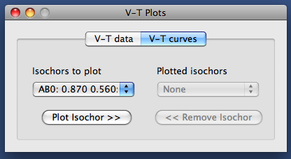
Selection of an isochor for plotting in a V-T diagram
FIT-Oil immediately plots the requested curve. In the example shown, the curve displays the typical convex-upward trend of an inclusion homogenising to liquid.
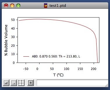
Example of a calculated V-T curve
8. To enter inclusion data
FIT-Oil provides an editor for entering microthermometric data for a series of petroleum inclusions.
To open an input window
- Select File > New...
- FIT-Oil displays the input window.
- Initially, the table contains a single row, each row corresponding to one inclusion.
- Enter:
- the homogenisation temperature Th in °C,
- the type of homogenisation (liquid or gas),
- the filling degree Fv in volume percent measured at a given temperature,
- the temperature at which the volume measurement was made,
- the mole percentages of CO2, N2, and H2S.
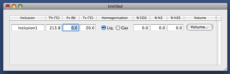
Input window for inclusion data
To add data for another inclusion
- Select Edit > Add a row... or use the shortcut Ctrl-K.
- A new empty row is added, in which the microthermometric and volumetric data can be entered.
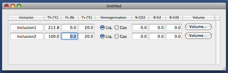
Adding a new inclusion row
To open an editor for volumetric data
- Click the Volume button at the end of the row.
FIT-Oil displays a new form window in which volumetric data can be entered.
The inclusion name appears in the window title. A first row is shown with two fields: T (°C) and % Gas, corresponding to the first V-T point.
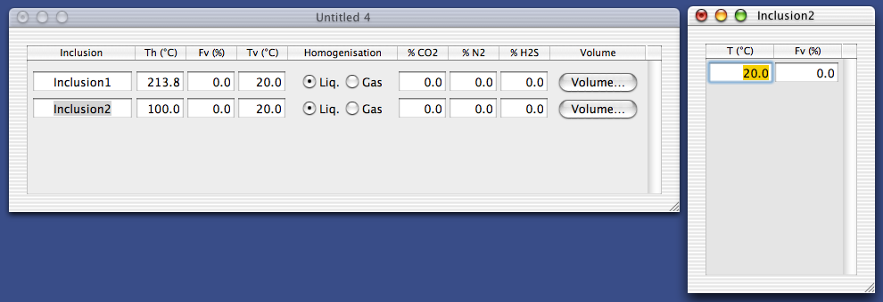
Volumetric data editor
To add volumetric data
- Use Ctrl-K or select Edit > Add a row... to append another row.
- Enter the bubble filling degree and the corresponding measurement temperature.
- Repeat the procedure for each volume-temperature measurement.
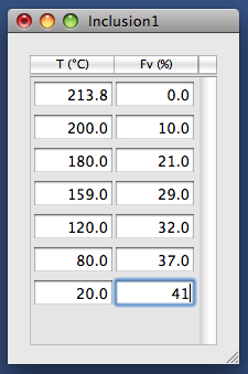
Additional volumetric data rows
9. To plot volumetric data
- Switch to the V-T data... panel of the V-T Plots floating window.
- The first list contains available inclusion data not yet plotted.
- The second list contains the inclusion data already added to the current V-T plot.
- Select the inclusion to plot in the first list.
- Click Plot Data >>.
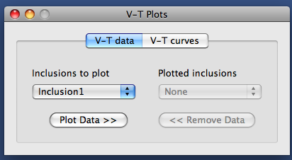
Plotting inclusion V-T data
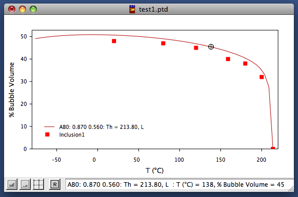
Inclusion V-T data displayed as solid squares
10. To define fluid models
In FIT-Oil, fluid models are user-defined compositional models, similar in spirit to those used in PVTSim. They are linked to thermodynamic models that allow the calculation of petroleum properties.
To open a fluid model data file
- Select Load Fluid Model... from the Fluid Model menu.
- A window opens. The left pane lists fluid models, while the right pane lists the components defined for the selected model.
- Other controls allow the user to adjust compositional parameters or select another thermodynamic model.
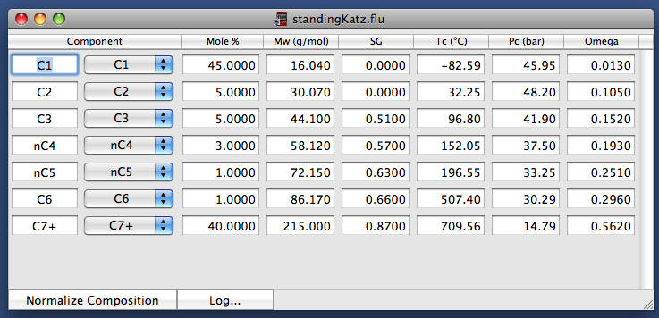
Fluid model editor window
To create a new fluid model data file
- Select New Fluid Model... from the Fluid Model menu.
- By default, only one fluid is defined, containing methane as a single component.
To add a fluid model
- Click the Add button.
- A new fluid model is created, initially containing only methane.
To delete a fluid model
- Select the fluid model in the left list.
- Click the Delete button.
To duplicate a fluid model
- Select the fluid model in the left list.
- Click the Duplicate button.
To select a compositional model
Each fluid model is defined by a compositional model, which determines the list of components and mole fractions. Several options are available:
- User defined: components and mole percentages are defined manually.
- Alpha-Beta model: uses the alpha-beta model implemented in FIT-Oil. Alpha and beta values can be entered directly or adjusted with stepper buttons.
- Alpha-Beta model (extended): an extended version using pseudo-components up to C40+.
- Gamma model: based on the model of Behrenbruch and Dedigama (2007) for crude oils. It uses three parameters: alpha, beta, and delta.
To visualize the composition spectrum
Use the plot displayed in the lower part of the window. By right-clicking in the plot area, several options become available:
- select a linear or logarithmic vertical scale,
- modify the upper bound of the vertical axis,
- display or hide a background grid,
- display data as bars, curves, or curves with markers,
- export the graphic as a PDF file,
- generate an Igor Pro text data file.
To modify a fluid model
In the editor window, all data can be modified. The meaning of the columns is as follows:
- SG: specific gravity,
- MW: molar mass,
- Tc: critical temperature in °C,
- Pc: critical pressure in bar,
- omega: acentric factor,
- Tb: boiling temperature in °C,
- Vc: critical molar volume in cm3/mol.
The first two columns give the component name (for example C1 for methane) or the fraction cut (for example C7+).
SG, MW, Tc, Pc, Tb, and omega can be adjusted for heavy fractions such as C7+ in order to improve the thermodynamic representation of selected properties, such as saturation pressure.
To change a component
A component can be changed in three ways:
- by typing its name into the Component field in the first column of the components table,
- by using the Component text field below the table,
- or, preferably, by selecting it from the pull-down menu.
After any component change, FIT-Oil automatically updates the corresponding SG, MW, Tc, Pc, and omega values. These values can then be edited manually if necessary.
To add a new component
- select Add row from the Edit menu,
- or use the shortcut Cmd-K,
- or click the Add button below the components table.
Note: this option is available only for user-defined compositional models.
To remove a component
- Select the component in the table.
- Select Delete row... from the Edit menu.
- FIT-Oil displays a confirmation dialog.
- Click OK to confirm.
11. To use a fluid model
To calculate properties under STP conditions
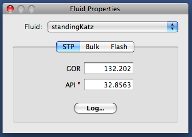
STP properties of a fluid model
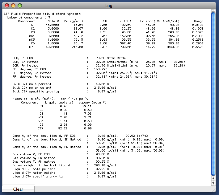
Additional STP properties window
To calculate bulk properties
Content not provided in the source.
To perform flash calculations
Content not provided in the source.
12. To generate a fluid model from an alpha-beta model
- Open the Alpha-Beta Plots floating window.
- Select the Fluids panel.
- Enter the alpha and beta parameters for your petroleum. You can use the spin boxes to adjust alpha and beta until the desired GOR and API° are reached.
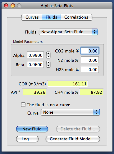
Selection of alpha and beta parameters
- Once the alpha and beta values have been chosen, click Generate Fluid Model...
- A new window opens, listing the pseudo-components, their mole percentages, and associated parameters.
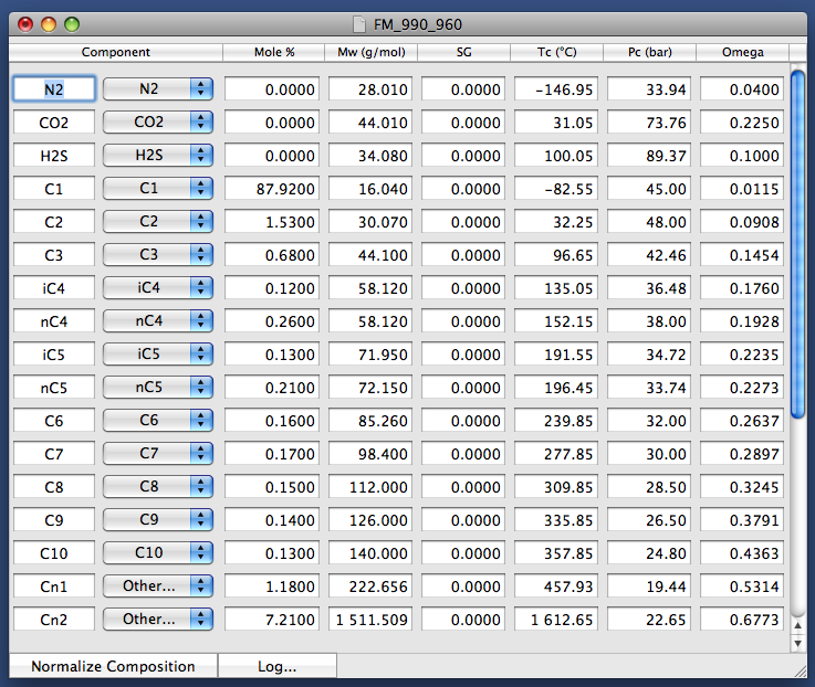
Fluid model generated from an alpha-beta model
Export results to Excel
All data and results used or produced by FIT-Oil can be exported to Microsoft Excel. This makes it possible to retrieve automatically the tables and figures generated by FIT-Oil, rework them, and print them.
- Open the worksheet FIT-Oil.xls located in the FIT-Oil.Excel folder.
- This workbook contains a series of macros.
- Excel displays a worksheet listing five main clickable topics:
- Read inclusion data: read a microthermometric data file,
- Read fluid model data: read a fluid model file,
- Read correlation data: retrieve alpha-beta correlations,
- View alpha-beta plot: read and process alpha-beta diagrams,
- View phase diagram: read and process P-T phase diagrams and V-T plots.
For each choice, Excel allows the user to select a FIT-Oil file and displays its content in a worksheet.
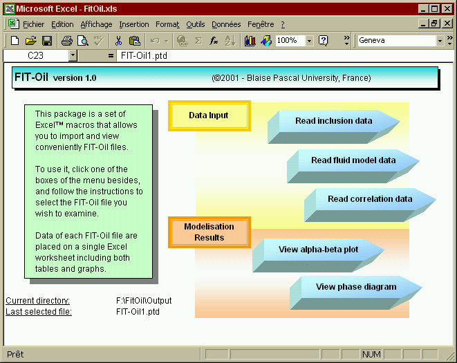
Excel main worksheet for FIT-Oil export
To import microthermometric and volumetric inclusion data
This Excel worksheet is used to import microthermometric and volumetric data for fluid inclusions.
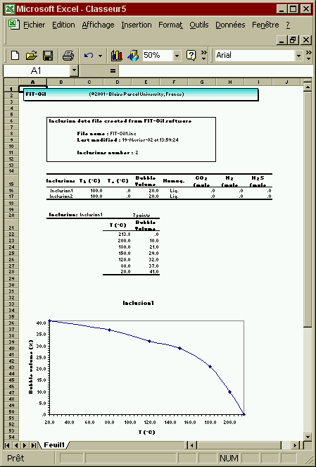
Excel worksheet for inclusion data import
To import fluid models
Fluid models are theoretical fluids described by 10 to 20 typical hydrocarbon components. They provide greater flexibility for describing the physico-chemical behaviour of petroleum.
The import worksheet includes:
- an upper section detailing fluid composition (component names and mole percentages),
- a lower bar chart visualising the composition of the model fluid.
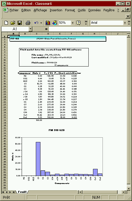
Excel worksheet for fluid model import
To import alpha-beta correlations
This worksheet is used to import alpha-beta correlations containing alpha-beta values for typical petroleums.
It presents successively:
- a table listing the petroleum types used in the correlation and their alpha-beta values,
- an alpha-beta diagram displaying the correlation,
- and, for each fluid, its theoretical composition as given by the alpha-beta model.
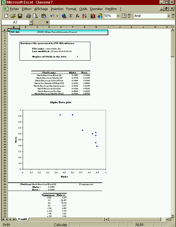
Excel worksheet for alpha-beta correlation import
To import alpha-beta plots
This worksheet is used to import an alpha-beta plot.
It presents successively:
- the alpha-beta plot with the calculated alpha-beta curves,
- and, for each alpha-beta curve:
- a table listing data such as inclusion name and homogenisation temperature,
- a table listing the alpha-beta values calculated for the curve.
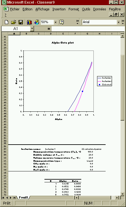
Excel worksheet for alpha-beta plot import
To import phase diagrams
This worksheet is used to import a phase diagram.
It presents successively:
- a header with general information such as the number of phase diagrams and the calculation date,
- and, for each imported phase diagram:
- the name of the phase diagram,
- the thermodynamic model used (fluid model or alpha-beta model),
- the fluid GOR,
- the list of pressure, temperature, and molar volume values along isopleths and isochores,
- and finally the trapping pressures estimated from homogenisation temperatures of aqueous inclusions and calculated isochores.
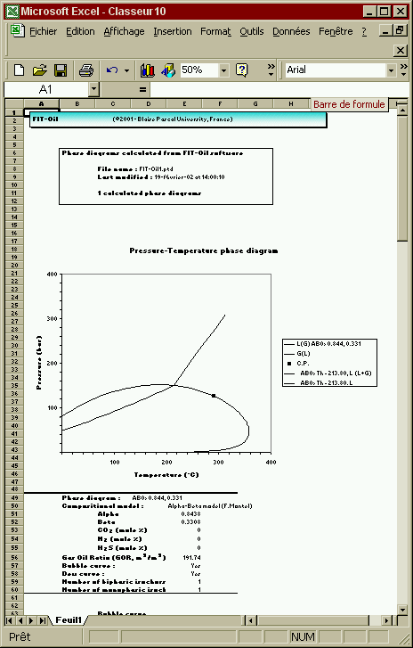
Excel worksheet for phase diagram import
The FIT-Oil user workspace
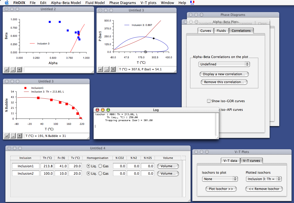
The FIT-Oil user workspace on Mac OS X
The FIT-Oil workspace is made up of several elements.
The menu bar
The menu bar includes six main menus:
- File,
- Edit,
- Alpha-Beta Model,
- Fluid Model,
- Phase Diagrams,
- V-T plots.
Data input windows
FIT-Oil provides several input windows for displaying and editing microthermometric data, alpha-beta correlations, and fluid models.
Diagrams
FIT-Oil mainly uses graphical representations to display calculation results. Plots are drawn for alpha-beta curves, phase diagrams, and bubble filling degree variations.
These graphical windows are more than simple plot viewers. Any displayed object (curve, point, axis, legend, etc.) can be selected with a mouse click. FIT-Oil then displays information about the selected object in floating windows.
Floating windows
FIT-Oil provides floating windows for displaying information and controls. Many tasks can be performed from these windows, especially those related to plots.
Three floating windows are used:
- one for alpha-beta diagrams,
- one for pressure-temperature phase diagrams,
- one for bubble-filling variation curves.
Contextual menus
Every graphical element in the diagrams can also be modified through contextual menus, accessible by right-clicking.
Menus
The following sections present the FIT-Oil menus in greater detail.
The Edit menu
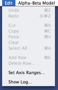
The Edit menu
The Edit menu contains general commands commonly found in many applications, such as Cut, Copy, and Paste.
Two additional menu items are also available:
- Add row: appends a new row in data input windows (microthermometric data, fluid model composition, petroleum compositions used in alpha-beta correlations, volumetric data),
- Delete row: removes a row. To delete a row, place the cursor in one of the text fields of that row.
Other menu items include:
- Set Axis Ranges...: displays a dialog box allowing the user to define axis ranges precisely,
- Show Log...: displays a text editor where FIT-Oil stores calculated results such as alpha-beta values or trapping pressures.
The Alpha-Beta Model menu
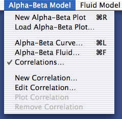
The Alpha-Beta Model menu
The Alpha-Beta Model menu provides access to commands for creating and modifying alpha-beta diagrams.
It includes:
- New (Alpha-Beta) Plot: creates a new alpha-beta document and displays an empty alpha-beta plot together with the corresponding floating window,
- Load (Alpha-Beta) Plot: loads and displays an existing alpha-beta plot document,
- Beta(Alpha) Curve...: displays the Curves panel of the floating window to calculate an alpha-beta curve,
- (Alpha-Beta) Fluid...: displays the Fluids panel to select an alpha-beta point and retrieve its properties; this panel also allows the generation of a fluid model,
- Correlations: displays the Correlations panel of the floating window to plot or remove correlations,
- New Correlation...: creates a new alpha-beta correlation document,
- Edit Correlation...: opens an existing alpha-beta correlation for editing,
- Plot Correlation...: plots a selected alpha-beta correlation in the current alpha-beta plot,
- Remove Correlation...: removes an alpha-beta correlation from the current alpha-beta plot.
The Fluid Model menu
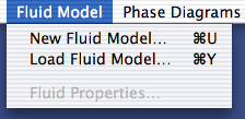
The Fluid Model menu
The Fluid Model menu provides access to commands for creating and editing fluid models.
It includes:
- New Fluid Model...: creates a new fluid model document,
- Load Fluid Model...: loads a fluid model document and displays it in an input window,
- Fluid Properties...: displays additional physico-chemical information about the petroleum, such as GOR and API°, and allows phase-equilibrium flash calculations.
The Phase Diagrams menu
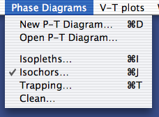
The Phase Diagrams menu
The Phase Diagrams menu provides access to commands for creating, calculating, and drawing phase diagrams in pressure-temperature space.
It includes:
- New P-T diagram...: creates a new phase diagram document and displays a new empty pressure-temperature plot together with the Phase Diagrams floating window,
- Open P-T diagram...: loads a phase diagram document and displays its contents,
- Isopleths...: displays the Isopleths panel of the floating window and allows the calculation of a new isopleth from an alpha-beta model or a fluid model,
- Isochors...: displays the Isochors panel and allows the user to add a new isochor,
- Trapping...: displays the Trapping panel and allows trapping pressures to be determined from isochores and aqueous inclusion homogenisation temperatures,
- Clean: displays the Clean panel, which allows various elements to be removed from the current phase diagram.
The V-T Plots menu
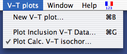
The V-T Plots menu
The V-T Plots menu provides access to commands for creating and modifying V-T plots, that is, bubble filling degree as a function of temperature.
It includes:
- New V-T plot: creates a new V-T plot,
- Plot Inclusion V-T Data: adds the Fv-T data of an inclusion,
- Plot Calc. V-T Isochor: adds the calculated bubble filling degree curve as a function of temperature.
Contextual menus
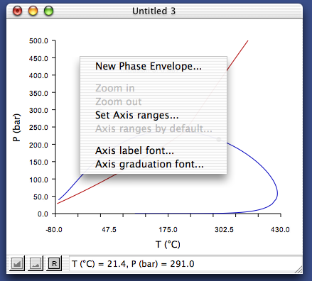
Contextual menu example
Every graphical object in a plot (curves, points, axes, etc.) has its own contextual menu, giving access to a set of related commands.
These contextual menus can be accessed by right-clicking the object to be modified.
For example, right-clicking on the background of a phase diagram displays the contextual menu associated with phase diagrams. This menu gives access, for example, to commands for calculating a new isopleth or modifying axis ranges.
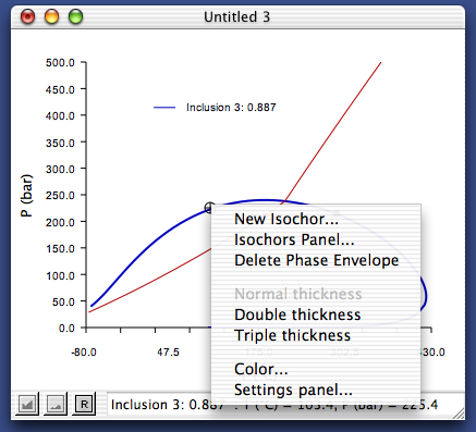
Contextual menus: isopleths
Contextual menu for isopleths
By right-clicking on an isopleth, the following actions become available:
- create an isochor homogenising at the point indicated by the mouse,
- delete the immiscibility loop indicated by the mouse, including any isochor or trapping line connected to it,
- modify the appearance of the curve, such as its width or colour.
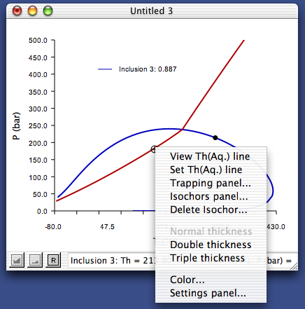
Contextual menus: isochores
Contextual menu for isochores
By right-clicking on an isochor, another contextual menu is displayed, allowing the user:
- to visualise the trapping line, that is, a vertical line intersecting the isochor at the trapping temperature,
- to fix a trapping line permanently,
- to access the Isochors or Trapping panels of the Phase Diagrams floating window,
- to remove the isochor from the diagram,
- to modify its appearance, such as line width or colour.
Publications
- [Thiéry, R., Pironon, J., Walgenwitz, F., Montel, F. (2002). Individual characterization of petroleum fluid inclusions (composition and P-T trapping conditions) by microthermometry and confocal laser scanning microscopy: implications for the applied thermodynamics of oils. Marine and Petroleum Geology, 19, 847-859.](download thiery2002.pdf)
- [Thiéry, R. (2006). Thermodynamic modelling of aqueous CH4-bearing fluid inclusions trapped in hydrocarbon-rich environments. Chemical Geology, 227, 154-164.](download thiery2006.pdf)
- [[Thiéry, R.]. A new object-oriented library for calculating high-order multivariable derivatives and thermodynamic properties of fluids with equations of state. Computers & Geosciences, 22 (1996), 801-815.
Download FIT-OIL
FIT-Oil is academic freeware and may be used and distributed free of charge.
- [FIT-Oil.dmg] — macOS version (Leopard; Intel and PowerPC). To install, open the disk image and drag the FIT-Oil application into your Applications folder.
- [FIT-Oil.exe] — Windows version.
- [FIT-Oil Excel Macros] — These macros have been tested on both macOS and Windows. However, depending on your version of Excel, some data conversion issues may occur.
- [FIT-Oil PDF] — A short introductory document presenting petroleum fluid inclusions and the main concepts used in FIT-Oil.