GEOD

Animation

Animations

A geological cross-section represents structures at a given instant t. To build it, one mainly relies on surface data, especially geological maps, but these data provide only a partial view of the underlying structures.

One way to reduce the uncertainty in reconstructing a cross-section is to imagine how the region looked before deformation. At that earlier stage, the structure was necessarily simpler, and GEOD provides the tools needed to reconstruct its subsequent deformation. This reconstruction may reveal folds or faults that must have developed through time.

This section reviews the main techniques available for moving and deforming structures through time.

Parameters varying through time

All the spatial characteristics of a point may vary through time. This includes coordinates, dips, and ranges. In every case, the syntax is similar. For example, for a line containing a moving point, one may write:

  line
      x 100 y 200
      x (200 at 0, 300 at 1) y 200

The values written in parentheses indicate that the second node of the line is located at x = 200 at t = 0, but at x = 300 at t = 1. The motion is linear.

A more complex motion, including changes in velocity, can also be defined:

  line
      x 100 y 200
      x (200 at 0, 300 at 1, 500 at 2) y (200 at 0, 100 at 1)

To simulate the formation of a fold with a Bézier curve, one could first write:

  bezier
      x 121.0 y 189.0
          range 100
          slope -45
      x (357.0 at 0, 300 at 1) y 193.0
          range 100
          slope -45
      graduate

This would produce something like the following:

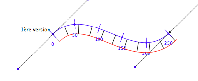
Figure 1: Initial state.

×

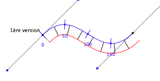
Figure 2: Final state.

In this example, only the x coordinate of the second node has been varied. One immediately notices that the length of the layer decreases from 250 to 150. In addition, the pattern tends to escape toward the right.

Other parameters must therefore be adjusted, for example the ranges of the nodes, so that the layer keeps a constant length. This adjustment is generally done step by step, by trial and error. One tests a value, then alternates between Command-0 and Command-1 to judge the result. One possible solution is:

  bezier
      x 121.0 y 189.0
          range (100 at 0, 150 at 1)
          slope -45
      x (357.0 at 0, 300 at 1) y 193.0
          range (100 at 0, 230 at 1)
          slope -45
      graduate

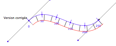
Figure 3: Initial state after adjusting the ranges.

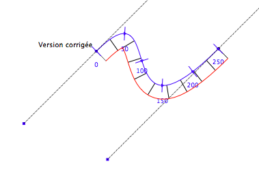
Figure 4: Final state after adjusting the ranges.

Using the graduate command, one can verify that the layer now keeps a constant length.

Curvilinear coordinates

Another way to introduce motion into a cross-section is to use curvilinear coordinates. This technique is especially useful when one block must slide relative to another. Full examples are given later. Here, only the syntax of the possible instructions is introduced.

The move command

The move command displaces a point along a given direction and over a given distance. It therefore plays a role similar to time-dependent coordinates such as x (...) and y (...), except that the movement is specified in polar form. The syntax is:

  line
      x 100 y 100
      move (0 at 0, 50 at 1) 45

Here, the first argument, (0 at 0, 50 at 1), gives the distance travelled by the point. In this example, the point moves 50 metres in one second. The second argument gives the direction of motion, here 45°.

The same conventions are used as for dip values:

• angles are measured clockwise,
• a value of 0 indicates a horizontal direction from left to right,
• a value of 180 indicates the opposite horizontal direction, from right to left.

Directions may also vary through time. For example, one may wish to prescribe the following motion: first, between t = 0 and t = 1, move 100 m horizontally from left to right; then, between t = 1 and t = 2, move 60 m upward along a 45° ramp; and finally, between t = 2 and t = 3, move another 50 m horizontally. Such a trajectory is typical of a point located at the leading edge of a thrust block moving up a ramp.

In GEOD, this motion could be written as:

  move (0 at 0, 100 at 1, 60 at 2, 50 at 3) (0 at 0, 0 at 0.999, 45 at 1, 45 at 1.999, 0 at 2)

An example of move is also given later for describing block displacement in an extensional setting.